The Mystique of the Smith Chart

I. The Smith Chart: A Navigator in the RF World

In the realm of RF transmission, the Smith Chart functions as a magical navigational tool, guiding engineers on their journey. Whether designing antennas or optimizing signal transmission, it is an indispensable ally.

Imagine designing antennas for 5G base stations; engineers strive for perfect matching network between antennas and feed lines to ensure maximum power transfer is efficiently utilized. Here, the Smith Chart, like an old friend, quietly aids in finding the optimal characteristic impedance matching solution. Within the analysis of RF circuits of a mobile phone, where signals must smoothly traverse between components, the Smith Chart helps adjust circuit parameters to minimize signal loss. What magic does it hold that grants it such high standing in RF engineering? Let's unveil Smith Chart‘s mysteries together.

II. The Birth of the Smith Chart

The Smith Chart was invented in 1939 by Phillip H. Smith, an innovator in the RF department at Bell Telephone Laboratories. After graduating from Tufts College, he honed his expertise in RF at RCA and Bell Labs. Legend has it that Smith often faced headaches dealing with complex calculations in transmission line problems. Traditional methods were time-consuming, labor-intensive, and prone to errors. During one infinite impedance matching study, pondering over a page full of formulas and data, he wondered if there could be a more intuitive and convenient method. Through persistent contemplation, he creatively transformed input reflection coefficients and impedance into a graphical calculator. This innovative idea made the previously esoteric transmission line calculations clear at a glance, opening a new door for RF engineers.

III. Components of the Smith Chart

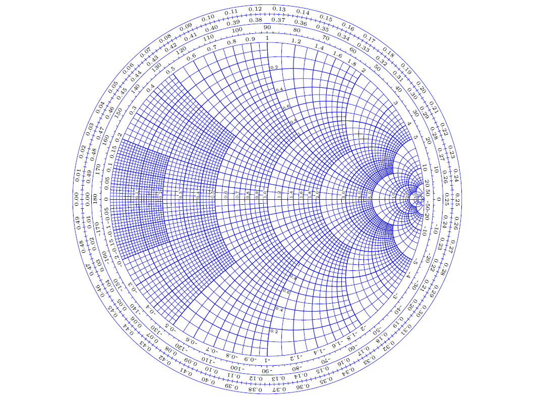
1. Constant Resistance Circles and Constant Conductance Circles: The Stable Foundation

Constant resistance circles form the foundation of the Smith Chart, representing stable resistance properties. Each unity circle signifies a fixed resistance value, akin to concentric tracks. By observing a blue circle, one can discern the corresponding input resistance which influences current and signal transmission.

Constant conductance circles offer insights into circuit characteristics from a conductance perspective, with their centers on the real axis. Larger conductance results in smaller circles. When handling parallel components, these outermost circles assist engineers in intuitively understanding conductance variations, optimizing circuit representation, and ensuring smooth signal transmission.

2. Constant Reactance Circles and Constant Susceptance Circles: The Dance of the Imaginative

Series reactance and constant susceptance circles resemble dancers, illustrating changes in reactance and susceptance on the Smith Chart. The upper half of constant reactance circles denotes inductive behavior, while the lower half indicates capacitive behavior. The susceptance circles are a "mirror image," with the upper half showing capacitive nature and the lower half inductive impedance. In analyzing common circuit elements, these circles interweave, allowing engineers to swiftly ascertain whether a circuit is inductive or capacitive and adjust parameters accurately.

3. Reflection Coefficient Family: The “Barometer” of Signal Reflection

The reflection coefficient family is crucial on the Smith Chart, acting as a "barometer" for signal reflection. The complex reflection coefficient plane, expressed as a complex number, represents the ratio of reflected to incident wave voltage and is depicted through concentric circles. A coefficient in terms of zero at the center signifies ideal matching, allowing unobstructed signal transmission; larger radii indicate higher reflection, with the largest radius reflecting complete wave reflection.

By examining intersection points of reflection coefficient scale with constant resistance and reactance circles, engineers can quickly assess circuit matching network levels. The reflection coefficient magnitude also relates to the Voltage Standing Wave Ratio (VSWR), a key measure of transmission line matching performance. On the Smith Chart, VSWR values can be estimated, evaluating line conditions to ensure efficient and stable signal transmission.

IV. Regional Characteristics of the Smith Chart

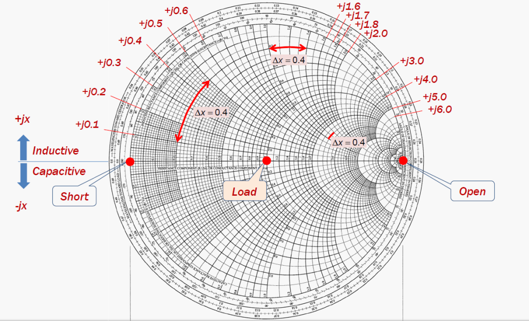
1. Dividing Inductive and Capacitive Regions

On the Smith Chart, the upper half-circle delineates inductive regions, while the lower half-circle illustrates capacitive regions. Connecting an inductor shifts the capacitive impedance trajectory clockwise upwards; attaching a capacitor moves it counterclockwise downwards. This facilitates instant identification of a circuit’s reactive component, providing guidance for parameter adjustments.

2. The Gradient "Spectrum" of Impedance Chart

Viewing the Smith Chart along the resistance axis reveals complex impedance values increasing like a spectrum. All circumferences intersect at a point on the real axis, with the largest circle representing pure reactance. As points move around the smith chart, each complete rotation corresponds to a change in electrical length, evoking a fascinating journey within the RF universe. This offers precise direction in understanding circuit input impedance characteristics.

V. Component Movements on the Smith Chart

1. Clockwise Rotation for Series Components

With series inductors, the inductive reactance is positive, causing an increase in inductive reactance and clockwise movement along a constant resistance circle, akin to an ascender climbing steadily. With series capacitors, the capacitive reactance is negative, decreasing capacitance reactance and moving the normalized impedance point counterclockwise, resembling a vessel gliding downstream.

2. Counterclockwise Rhythm for Parallel Components

For parallel inductors or capacitors, observations are made using the admittance chart. With parallel inductors, the imaginary part of normalized admittance decreases, moving the impedance point counterclockwise along a constant conductance circle, much like a dancer gracefully twirling. Parallel capacitors increase the imaginary part of admittance, shifting the point clockwise like unlocking a new doorway.

VI. Practical Use of the Smith Chart: The Art of Impedance Matching

1. The Significance of Impedance Matching

Impedance matching acts as a bridge, connecting signal sources and arbitrary loads to ensure efficient energy transfer. Mismatches lead to energy reflections, reducing efficiency and affecting system stability. Proper matching allows for smooth energy transfer, unleashing optimal performance.

2. Practical Case Study

Consider an RF transmission circuit with known source impedance, load impedance, transmission line characteristic impedance, and frequency of operation. After normalizing impedances, locate the corresponding point on the Smith Chart. With the load impedance being capacitive, first parallel an inductor to move the impedance point counterclockwise near the center; then series a capacitor to shift the point clockwise towards the center, achieving matching. Post-adjustment, maximum power transfer efficiency significantly increases, minimizing signal reflection and ensuring stable circuit manipulation.

Over the years, the Smith Chart remains a graphical tool in the RF field, demonstrating robust adaptability from basic circuit design to cutting-edge technology. Delving into the Smith Chart is essential for exploring the RF domain. As technology advances, the Smith Chart will continue to evolve, injecting fresh vitality into the RF landscape.