1. What is an oscilloscope?
An oscilloscope is a very versatile electronic measuring instrument. It can transform invisible electrical signals into visible images, making it easy for people to study the process of various electrical phenomena. Oscilloscopes utilize a narrow, high-speed electron beam composed of electrons, which hits the screen surface coated with fluorescent material, producing a small point of light. Under the action of the measured signal, the electron beam resembles the tip of a pen, capable of depicting the change curve of the instantaneous value of the measured signal on the screen surface. It has critical applications in various fields, including electronics, electrical engineering, communications, and computers, such as observing signal wave forms, measuring frequency, amplitude, phase, and other signal parameters, and providing a powerful tool for debugging, troubleshooting, and scientific research of circuits.
Composition of oscilloscope
Oscilloscope: The Oscilloscope is the core part of the oscilloscope, composed of an electron gun, a deflection system, and a fluorescent screen. The electron gun launches an electron beam, which is controlled by the deflection system and hits the fluorescent screen to form a light spot. The phosphor screen is coated with a fluorescent substance that glows when the electron beam hits it, creating a visible waveform.
Vertical (Y-axis) Amplifier Circuit: Amplifies the input signal to display the appropriate amplitude on the phosphor screen.
Horizontal (X-axis) Amplifier Circuit: Generates a sabretooth wave scanning signal, which is used to control the horizontal scanning of the electron beam on the phosphor screen to display the time axis of the signal.
Scanning and Synchronization Circuit: generates the sabretooth wave voltage to form the time baseline of the electron beam on the fluorescent screen and ensures that the scanning of the electron beam is synchronized with the frequency and phase of the input signals to display the waveform of the signals correctly.
Power supply circuit: provides the required power supply for each part of the oscilloscope, including high-voltage power supply, filament power supply, etc.
Probe: usually divided by the measurement object, there are two kinds of voltage probes and current probes. Voltage probes include passive probes and active probes. Passive probes in the 1X, 10X, 100X, and 1000X ranges can measure up to 40KV at high voltage. Active probes, which include both ordinary and differential types, are primarily used. For the active probes, the maximum safety voltage limit is often tens of volts. To avoid personal safety hazards and the potential danger of damaging probes, it is essential to know the voltage range being measured and the voltage limits of the probes to be used. Active differential probes help you observe differential signals. Differential signals are signals referenced to each other, not to ground. Differential probes have higher performance when used with matched pairs of single-ended probes, providing high CMRR, wide bandwidth, and minimal time differences between input signals. High bandwidth differential probes provide excellent signal fidelity to meet the needs of engineers and technicians designing and debugging at fast clock rates and clock edge rates. Current probes include AC probes and AC/DC probes. AC probes are usually passive probes, and AC/DC probes are usually active probes.
2. Types of oscilloscopes
Oscilloscopes are generally divided into analog oscilloscopes and digital oscilloscopes. While both can be used for testing, analog oscilloscopes are typically preferred for signals that require real-time display and change rapidly, as well as for complex signals. Digital oscilloscopes are used to display the periodicity of relatively strong signals, including both digital and analog signals. Their built-in CPU or special digital signal processor enables the analysis of signals and the saving of wave forms, providing significant convenience during analysis and processing.
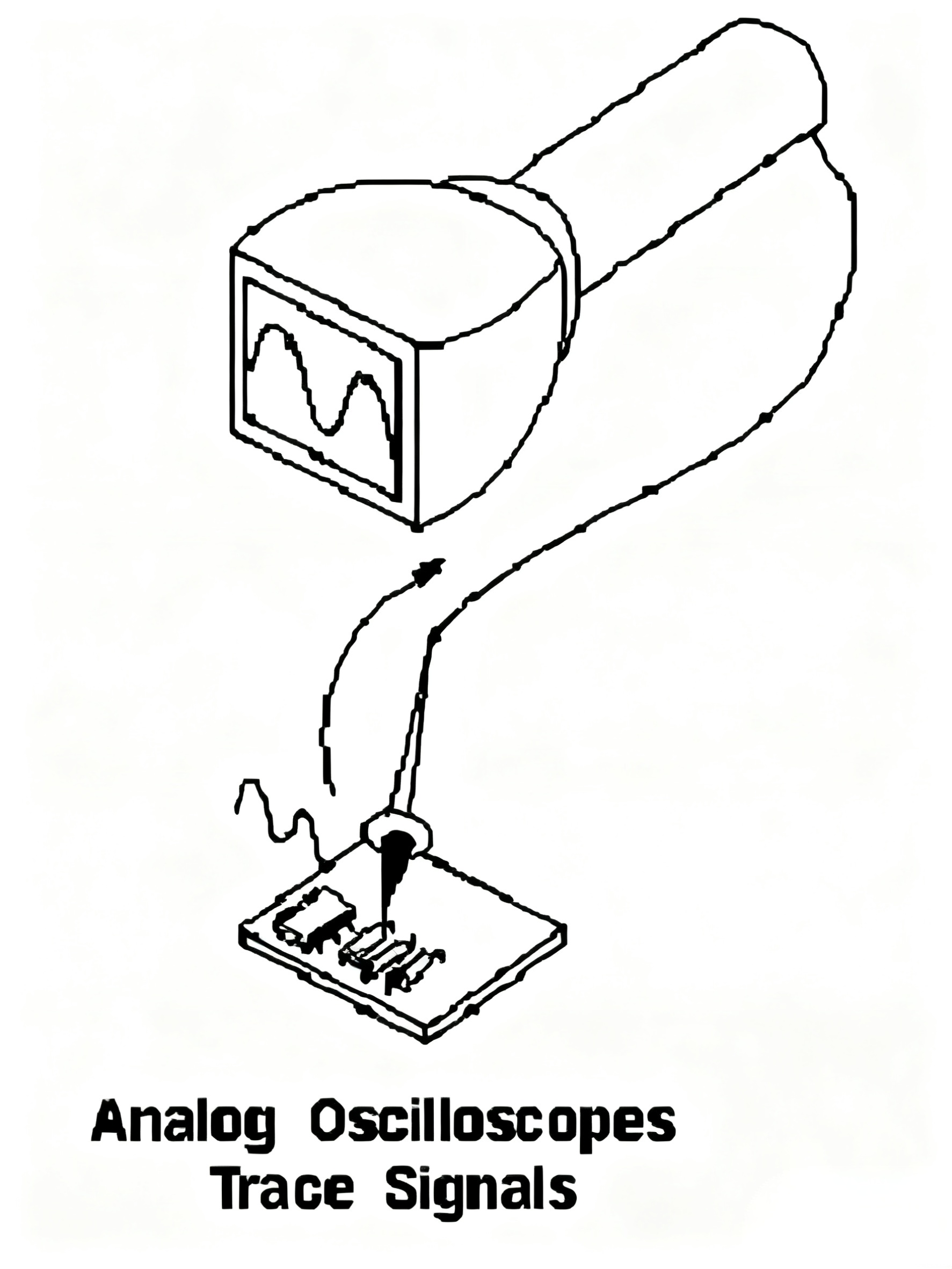
2.1 Analog Oscilloscope
An analog oscilloscope uses an electron gun to scan the screen of the oscilloscope, with deflection voltage, so that the electron beam scans uniformly from top to bottom, and the waveform will be displayed on the screen. Its advantage lies in the real-time display of images.
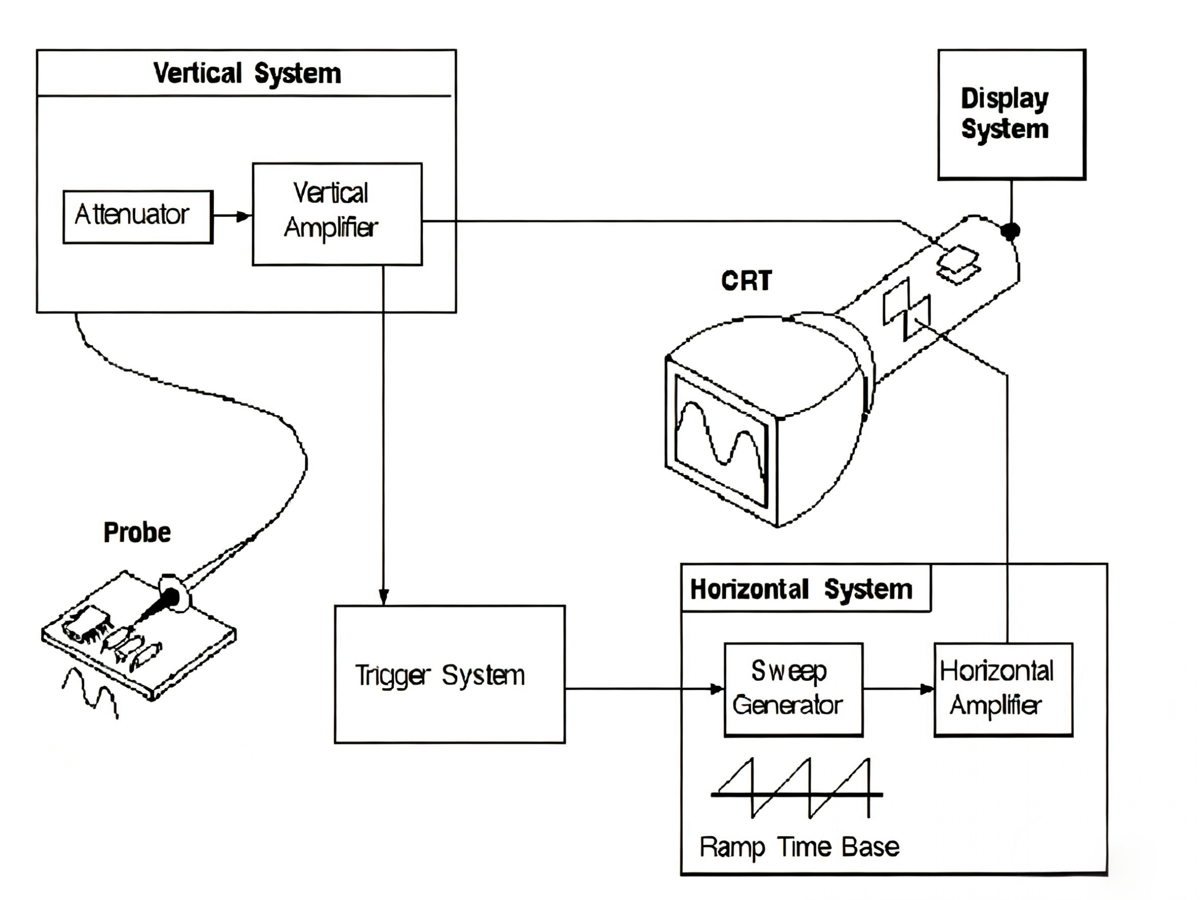
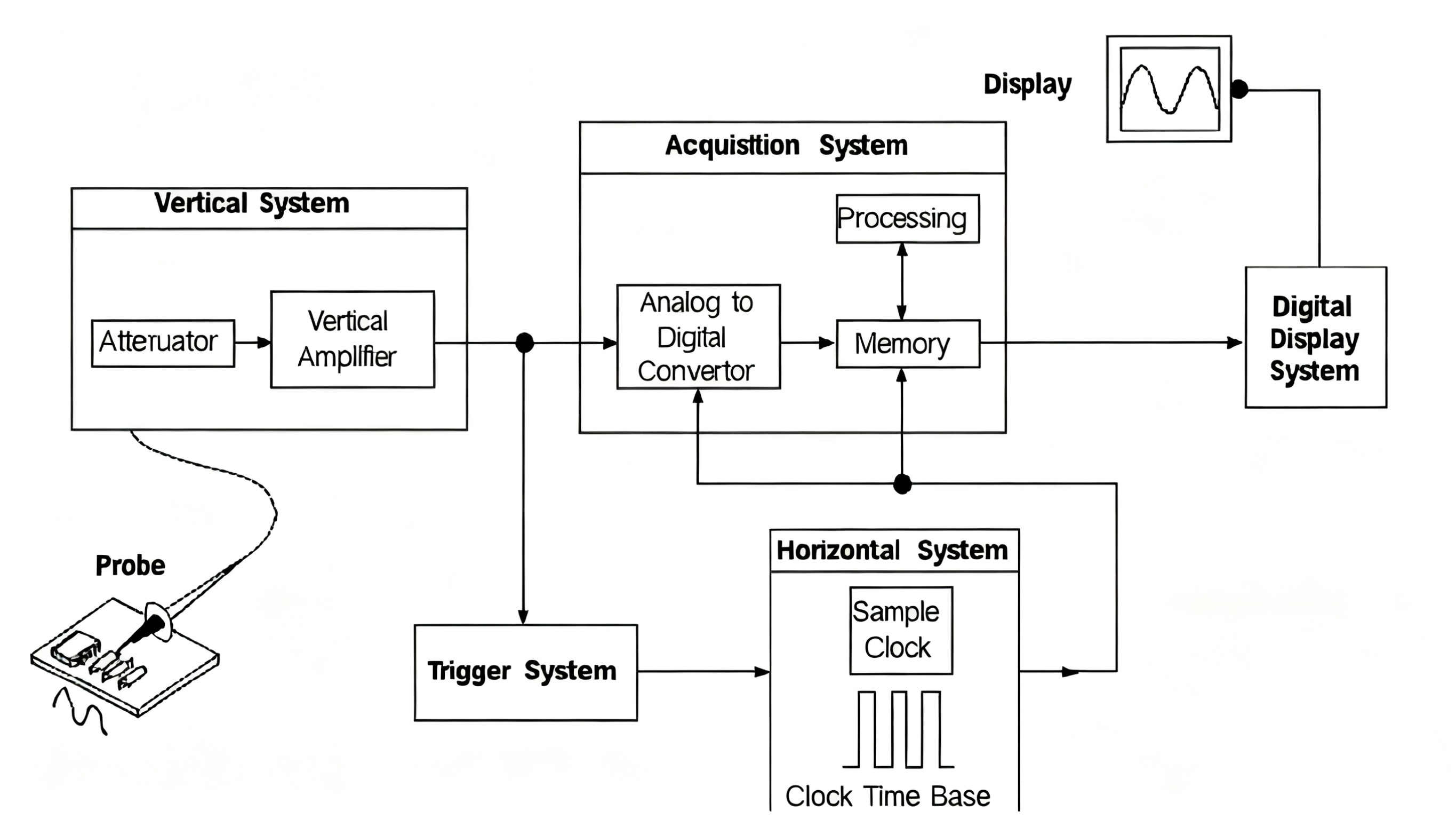
The block diagram of an analog oscilloscope is shown below:
The above diagram shows that the signal under test is processed by the vertical system (such as attenuation or amplification, i.e., we screw the vertical button -volts/div), and then sent to the vertical deflection control. And the trigger system will control the generation of the horizontal scanning voltage (sabretooth wave) to be sent to the horizontal deflection control, depending on the trigger setting.
The signal arrives at the trigger system and starts or triggers a "horizontal scan", which is a sabretooth wave that scans the dot horizontally. Triggering the horizontal system produces a horizontal time base that causes the dot to scan from the left to the right side of the screen in a precise amount of time. The fast scanning process will make the motion of the dot look like a smooth curve. The signal voltage applied to the electrodes of the vertical deflection voltage also has the effect of creating a moving dot. A positive voltage will move the dot upward, a negative voltage will move it downward, and the horizontal and vertical deflection voltages together will be able to display the waveform of the signal on the screen. At a relatively high speed, the bright spot can scan across the screen up to 50,000 times/second. In contrast, the best general-purpose oscilloscope can only capture 40,000 waveforms per second. This makes analog oscilloscopes more real-time than digital oscilloscopes, which is the real deal.
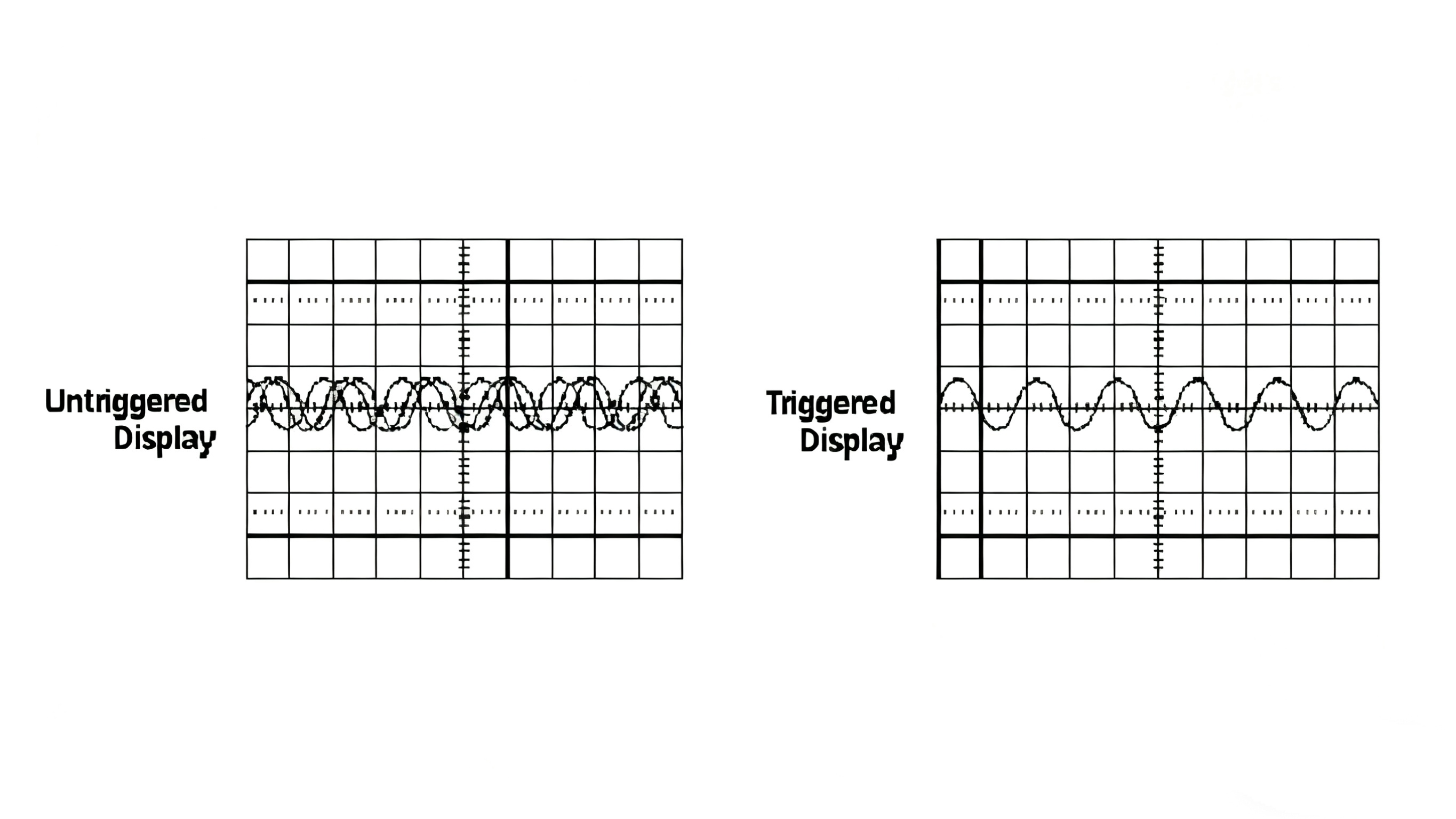
Horizontal scanning and vertical deflection enable the waveform image of a signal to be displayed on the screen, however a trigger system is also essential, not only does it allow you to capture the waveform you need, but it also enables the image to be displayed on the screen stably, it enables repetitive wave forms to be scanned at the same point to start the scanning process, displaying a clean and stable image on the screen.
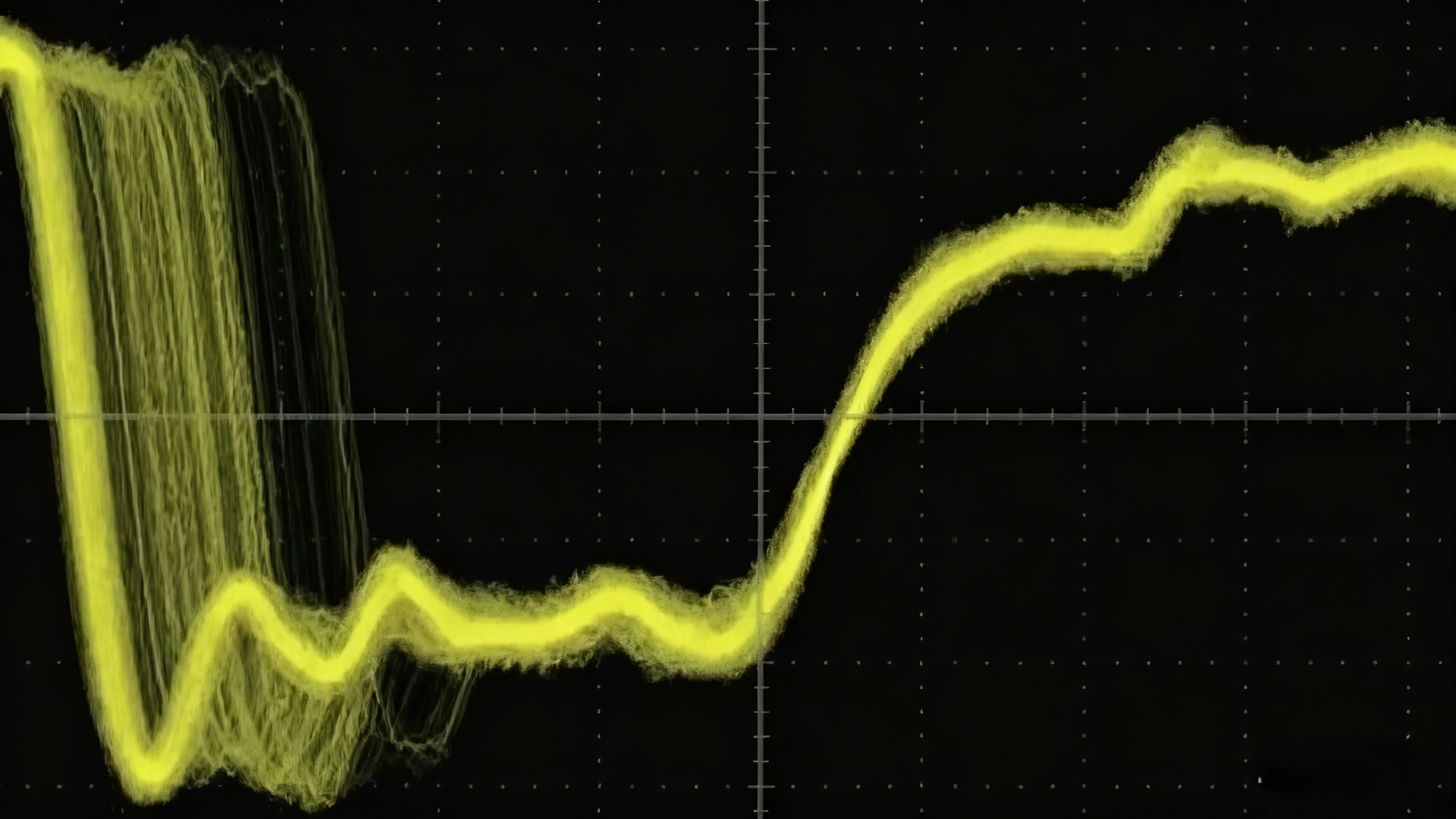
The photo below shows the intrigued and triggered wave forms: the intrigued waveform is messy, flickering, and unstable, while the triggered waveform is very stable and clean.
Generally speaking, with an analog oscilloscope, we need to adjust three fundamental aspects, the three parts mentioned above:
The attenuation or amplification of the signal: using the volts/div knob, you can adjust the signal to be inside the scope of the screen, with the correct vertical size.
Time base: Using the sec/div knob, the time interval represented by each frame can be adjusted to make the signal zoom in or out horizontally.
Trigger system: You can adjust the trigger level to stabilize the waveform display or locate the desired waveform.
Of course, adjusting the size of the bright spot and the bright bottom can make the waveform display achieve the best display effect.
2.2 Digital Oscilloscope
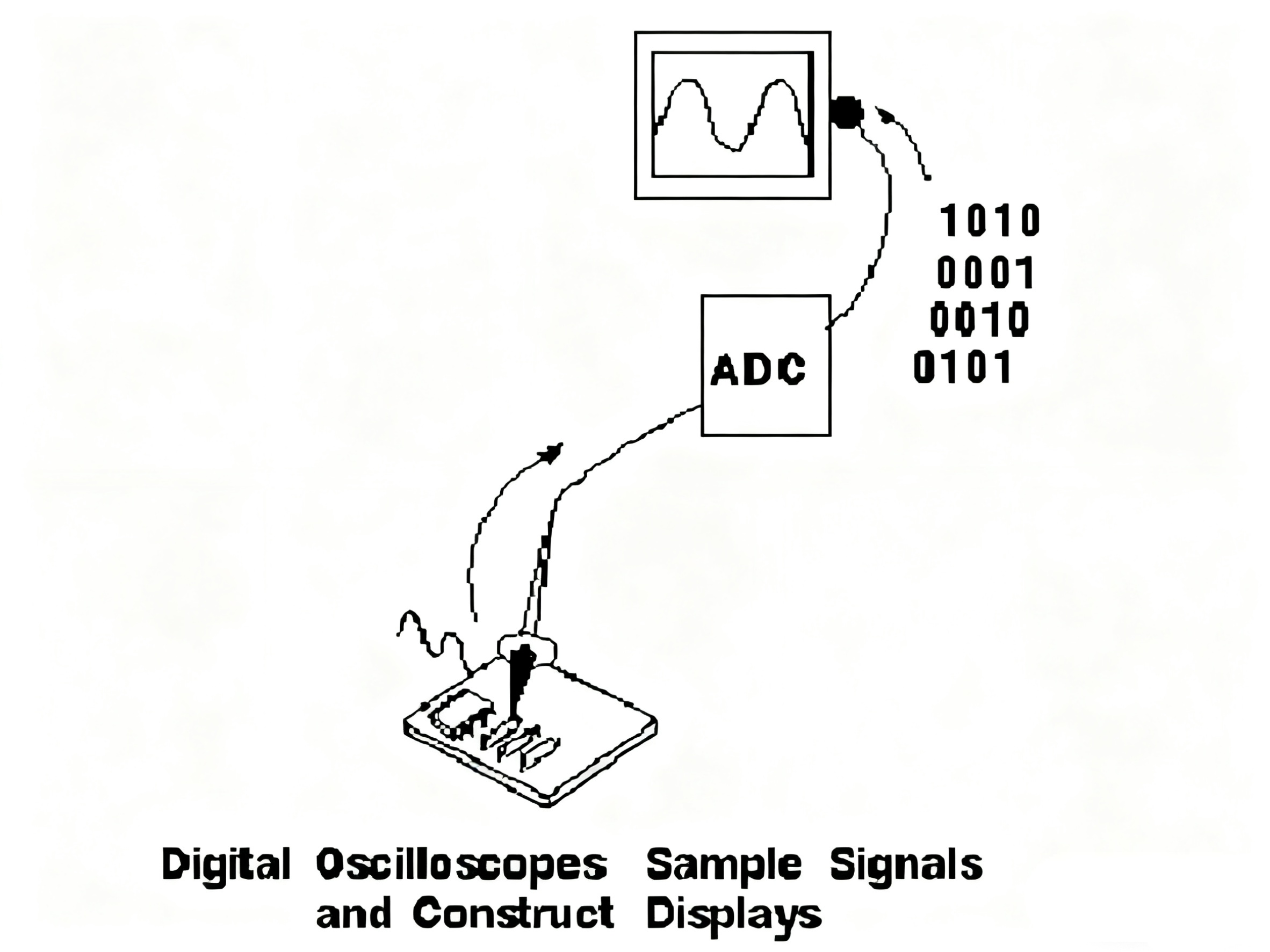
A digital oscilloscope samples the wave forms and uses an ADC to convert the analog image to digital wave forms, and finally reproduces the wave forms on the screen.
The schematic diagram of a digital oscilloscope is shown below:
When we connect the probe to the top of the line, the vertical system controls the adjustment of the attenuation and amplification of the signal, which is the same as that of the analog oscilloscope. Next, the analog-to-digital conversion (ADC) is performed on the signal in the sampling system, and the continuous analog signal becomes discrete dots. The time base of the level system determines the level of the sampling rate.
For example, our TDS5054 has a maximum sampling rate of 5GSa/s, indicating that it is capable of sampling 5G points per second at its fastest. The sampled and antiquated points are stored in memory and pieced together into a waveform graph.
In digital oscilloscopes, the length of the stored waveform points is often referred to as the memory length. Due to their high-speed processing requirements, these memories are not general-purpose Dramas but specialized high-speed memories, which are more expensive; therefore, cheaper oscilloscopes use standard configurations. The trigger system determines the start and end points of the save point. The wave forms inside the memory are finally transferred to the display system for display.
Data processing is necessary to enhance the oscilloscope's synthesizing power. In addition, ore-triggering enables us to see the waveform before triggering.
As with analog oscilloscopes, testing with a digital oscilloscope requires adjusting the vertical amplitude, horizontal time interval, and trigger settings.
3. How does an oscilloscope work?
An oscilloscope is an electronic measuring instrument that utilizes the characteristics of an electronic oscilloscope to convert alternating electrical signals, which are not directly observable by the human eye, into an image that is displayed on a fluorescent screen for measurement. It is an essential instrument for observing the experimental phenomena of digital circuits, analyzing the problems in the experiments, and measuring the experimental results. The oscilloscope consists of an oscilloscope and power supply system, a synchronization system, an X-axis deflection system, a Y-axis deflection system, a delay scanning system, and a standard signal source.
3.1 Fluorescent screen
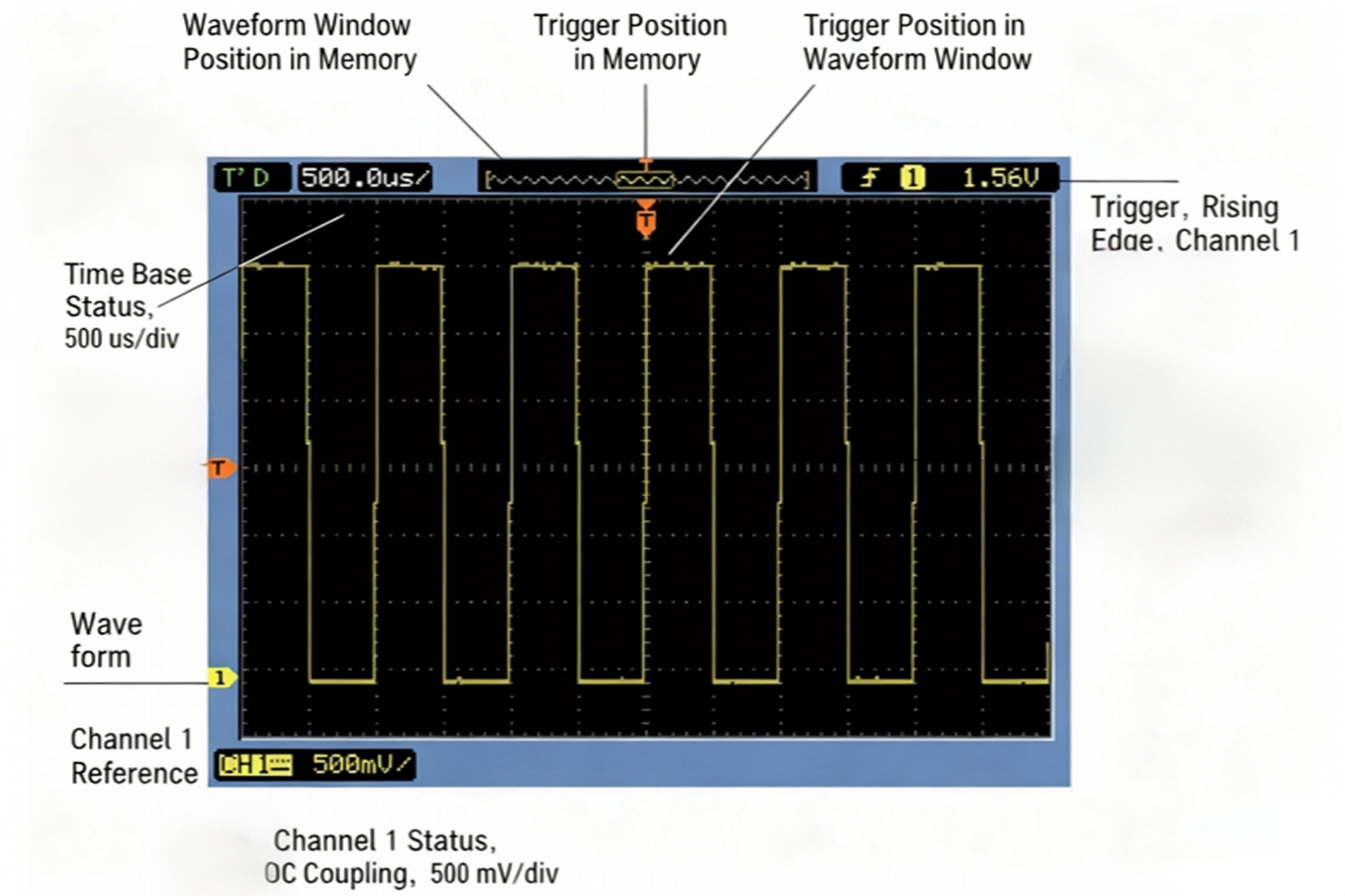
The fluorescent screen is the display part of the oscilloscope. There are several scale lines on the screen in the horizontal and vertical directions, indicating the relationship between voltage and time of the signal waveform. The horizontal direction indicates the time, and the vertical direction indicates the voltage. The horizontal direction is divided into 10 frames, and the vertical direction is divided into eight frames, each of which is further divided into five parts. Vertical direction is marked with 0%, 10%, 90%, 100%, etc. The horizontal direction is marked with 10% and 90% for measuring DC level, AC signal amplitude, delay time, and other parameters. According to the measured signal on the screen, the number of frames can be derived from the voltage value and time value by multiplying by the appropriate constant of proportionality (V / DIV, TIME / DIV).
3.2 Oscilloscope and power system
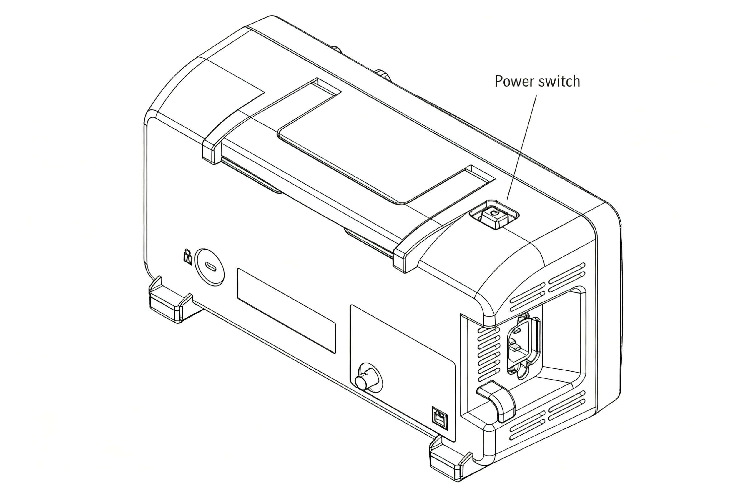
(1) Power supply (Power)
The oscilloscope's main power switch. When this switch is pressed, the power indicator lights up, indicating that the power supply is on.
(2) Glow (Intensity)
Rotate this knob to change the brightness of the light spot and scan line. Observe that low-frequency signals can be smaller, high-frequency signals larger.
Generally, it should not be too bright to protect the fluorescent screen.
(3) Focus
The focus knob is used to adjust the size of the electron beam cross-section, and the scanning line will be focused into the clearest state.
(4) Scale brightness (Illuminance)
This knob adjusts the brightness of the illuminate behind the fluorescent screen—normal indoor light results in darker illumination. In an environment with insufficient indoor light, the illumination can be adjusted appropriately.
3.3 Vertical deflection factor and horizontal deflection factor
(1) Vertical Deflection Factor Selection (VOLTS/DIV) and Fine Tuning
Under the action of the unit input signal, the distance that the point of light is deflected on the screen is called the offset sensitivity, and this definition applies to both the X-axis and the Y-axis. The reciprocal of the sensitivity is called the deflection factor. Vertical sensitivity is measured in cm/V, cm/V, or DIV/V, DIV/V, and vertical deflection factor is measured in V/cm, V/cm, or V/DIV, V/DIV. In fact, the deflection factor is sometimes used as the sensitivity due to customary usage and the convenience of measuring voltage readings.
Each channel of the oscilloscope has a vertical deflection factor selector switch. The band switches are generally divided into 10 steps from 5mV/DIV to 5V/DIV in 1, 2, and 5 steps. The value indicated by the band switch represents the voltage value of the vertical direction of a frame on the fluorescent screen. For example, when the band switch is placed in 1V / DIV gear, if the signal light point on the screen moves by one frame, it represents a 1V change in the input signal voltage.
There is often a small knob on each band switch to fine-tune the vertical deflection factor of each gear. Turn it clockwise to the end, in the "calibration" position, when the vertical deflection factor value is the same as the value indicated by the band switch. Turn this knob counterclockwise to fine-tune the vertical deflection factor. It should be noted that the fine adjustment of the vertical deflection factor may cause inconsistency with the value indicated by the band switch. Many oscilloscopes have a vertical expansion function, which expands the vertical sensitivity (and reduces the deflection factor) by a factor of several when the fine adjustment knob is pulled out. For example, if the deflection factor indicated by the band switch is 1V/DIV, the vertical deflection factor is 0.2V/DIV when the ×5 expansion state is used.
When doing digital circuit experiments, the ratio of the vertical travel distance of the measured signal on the screen to the vertical travel distance of the +5V signal is often used to determine the voltage value of the measured signal.
(2) Time Base Selection (TIME/DIV) and Trimming
Time base selection and trim are used in a similar way to vertical deflection factor selection and trim. The time base selection is also realized by a band switch, which divides the time base into several steps, such as 1, 2, and 5. The indication value of the band switch represents the time value for the point of light to move horizontally by one frame. For example, in the 1μS/DIV mode, the point of light moving one frame on the screen represents a time value of 1μS.
The "Trim" knob is used for time base calibration and trimming. When the knob is rotated clockwise to the calibration position, the time base value displayed on the screen corresponds to the nominal value indicated by the band switch. Turning the knob counterclockwise fine-tunes the time base. When the knob is removed, it is in the scanning expansion state. For example, at 2μS/DIV, the time value represented by one horizontal frame on the fluorescent screen in the scanning expansion state is equal to
2μS×(1/10)=0.2μS
There are 10MHz, 1MHz, 500kHz, and 100kHz clock signals on the TDS test bench, which are generated by a quartz crystal oscillator and a frequency divider with high accuracy, and can be used to calibrate the time base of the oscilloscope.
The oscilloscope's standard signal source, CAL, is specifically designed to calibrate the oscilloscope's time base and vertical deflection factor. For example, the COS5041 oscilloscope standard signal source provides a square wave signal with VP=2V and f=1kHz.
The Position knob on the front panel of the oscilloscope adjusts the position of the signal waveform on the fluorescent screen. Rotate the horizontal displacement knob (labeled with horizontal two-way arrow) to move the signal waveform left and right, and rotate the vertical displacement knob (labeled with vertical two-way arrow) to move the signal waveform up and down.
3.4 Input channel and input coupling selection
(1) Input channel selection
There are at least three ways to select the input channel: channel 1 (CH1), channel 2 (CH2), and dual channel (DUAL). When channel one is selected, the oscilloscope only displays the signal of channel 1. When Channel 2 is selected, the oscilloscope only displays the signal of Channel 2. When selecting DUAL, the oscilloscope displays the signals of channel one and channel two simultaneously. To test the signals, first connect the ground of the oscilloscope to the ground of the circuit under test. According to the selection of the input channel, plug the oscilloscope probe into the corresponding channel socket. The ground on the oscilloscope probe is connected to the ground of the circuit under test, and the oscilloscope probe touches the point under test. The oscilloscope probe has a two-position switch. This switch is dialed to the "× 1" position, the measured signal is sent to the oscilloscope without attenuation, and the voltage value read out from the fluorescent screen is the actual voltage value of the signal. This switch is dialed to the "× 10" position, the measured signal attenuation for 1 / 10, and then sent to the oscilloscope. From the fluorescent screen, read out the voltage value multiplied by 10, which is the actual voltage value of the signal.
(2) Input coupling method
Input coupling mode has three options: alternating current (AC), ground (GND), and direct current (DC). When "Ground" is selected, the scan line shows the position of "Oscilloscope Ground" on the fluorescent screen. DC coupling is used to determine the absolute DC value of signals and to observe very low-frequency signals. AC coupling is used to observe AC and DC signals. In digital circuit experiments, the general choice of "DC" mode is made to observe the absolute voltage value of the signal.
3.5 Triggering
After the measured signal is input from the Y-axis, a part of it is sent to the Y-axis deflection plate of the oscilloscope to drive the light point to move along the vertical direction on the fluorescent screen according to the ratio; another part of it is shunted to the x-axis deflection system to generate a trigger pulse, which triggers the scanning generator and produces a repetitive sabretooth voltage added to the X-axis deflection plate of the oscilloscope to make the light point to move along the horizontal direction.
The two of them are combined, and the light point is depicted in the graphic on the fluorescent screen, that is, the graphic of the measured signal. The graph shown by the light spot on the fluorescent screen is the measured signal graph. It can be seen that the correct trigger mode directly affects the effective operation of the oscilloscope. To achieve a stable and transparent signal waveform on the fluorescent screen, mastering the basic trigger function and its operation is crucial.
(1) Trigger source selection
To make the screen display a stable waveform, it is necessary to measure the signal itself, or to measure the signal with a specific time relationship with the trigger signal added to the trigger circuit. Trigger source selection determines where the trigger signal is supplied. There are usually three trigger sources: internal trigger (INT), power trigger (LINE), and external trigger EXT).
The internal trigger uses the signal under test as the trigger signal and is a frequently used trigger method. Since the trigger signal itself is part of the signal under test, a very stable waveform can be displayed on the screen. Channel 1 or channel 2 in dual-trace oscilloscopes can be selected as the trigger signal.
Power triggering uses the AC power supply frequency signal as the trigger signal. This method is effective in measuring signals related to the AC power supply frequency. It is especially effective in measuring low-level AC noise in audio circuits and gate tubes.
External triggering uses an external signal as the trigger signal, which is input from the external trigger input. There should be a periodic relationship between the external trigger signal and the measured signal. Since the signal under test is not used as the trigger signal, the scanning start time is independent of the signal under test.
The correct selection of the trigger signal has a great deal to do with the stability and clarity of the waveform display. For example, in the measurement of digital circuits, for a simple periodic signal, the choice of internal triggering may be better. In contrast, for a signal with a complex cycle and a periodic relationship, the choice of external triggering may be better.
(2) Trigger coupling mode selection
Trigger signals to the trigger circuit of the coupling method can be achieved in various ways. The purpose is to ensure signal stability and reliability. Here are a few commonly used.
AC coupling is also known as capacities coupling. It allows only the AC component of the trigger signal to be triggered, and the DC component of the trigger signal is isolated. This type of coupling is usually used when the DC component is not considered to form a stable trigger. However, if the frequency of the trigger signal is less than 10 Hz, it can cause triggering difficulties.
Direct current coupling (DC) does not isolate the DC component of the trigger signal. When the frequency of the trigger signal is low or the duty cycle of the trigger signal is large, it is better to use DC coupling.
When the trigger signal is triggered by low frequency rejection (LFR), the trigger signal is added to the trigger circuit through a high-pass filter, and the low-frequency component of the trigger signal is suppressed; when the trigger signal is triggered by high frequency rejection (HFR), the trigger signal is added to the trigger circuit through a low-pass filter, and the high-frequency component of the trigger signal is suppressed. In addition, there is a TV synchronization (TV) trigger for TV maintenance. These trigger coupling methods have their own scope of application and require experience in use.
(3) trigger level and trigger polarity (Slope)
Trigger level adjustment, also known as synchronization adjustment, synchronizes the scanning and the measured signal. The level adjustment knob adjusts the trigger level of the trigger signal. Once the trigger signal exceeds the trigger level set by the knob, the scan is triggered. Turning the knob clockwise increases the trigger level; counterclockwise decreases the trigger level. When the level knob is adjusted to the level lock position, the trigger level is automatically kept within the amplitude of the trigger signal, and a stable trigger can be generated without level adjustment. When the signal waveform is complex, the level knob can not stabilize the trigger. Use the release suppression (Hold Off) knob to adjust the release suppression time of the waveform (scanning pause time), which can make the scanning and the waveform stabilization in sync.
The polarity switch is used to select the polarity of the trigger signal. When the switch is set to the "+" position, the trigger will be generated when the trigger signal exceeds the trigger level in the direction of signal increase. In the "-" position, the trigger is generated when the trigger signal exceeds the trigger level in the direction of signal decrease. Trigger polarity and trigger level together determine the trigger point of the trigger signal.
3.6 Scanning mode (Sweep Mode)
Scanning has three kinds of scanning modes: automatic (Auto), standard (Norm), and single (Single).
Auto: When there is no trigger signal input, or the trigger signal frequency is lower than 50Hz, the scanning is in self-excited mode.
Normal: When there is no trigger signal input, the scanning is in the ready state, and there is no scanning line. When the trigger signal arrives, the scan is triggered.
Single: The single button is similar to the reset switch. Under the single scanning mode, the scanning circuit is reset when the single button is pressed, and the Ready light is on at this time. A single scan is generated when the trigger signal arrives. When the single scan is finished, the Ready lamp goes out. A single scan is used to observe non-periodic signals or single transient signals, which often require taking pictures of the waveform.
4. What is an oscilloscope used for?
4.1 Three major applications of oscilloscopes
(1) Oscilloscope Application 1
Debugging of general-purpose signals, waveform observation and measurement of basic waveform parameters, circuit diagnosis, and capture of anomalies. Using an oscilloscope to test a circuit is actually similar to using a altimeter to test a circuit. Knowing the general voltage of the circuit, you can quickly find the problem based on the voltage. Know what kind of wave forms are being measured, and compare them.
(2) Oscilloscope Application 2
Advanced analysis of signals enables the decoding of serial signals from the content carried vertically. An eye diagram is a series of digital signals displayed on the oscilloscope's cumulative graphic display. It contains a wealth of information that can be observed with the eye on the crosstalk between the code and the impact of noise, reflecting the overall characteristics of the digital signal, to estimate the extent of the system's strengths and weaknesses.
(3) Oscilloscope Application 3
In the modulation domain analysis of ultra-waveband signals, you can use the spectrometer as a down converter, with a UWB bandwidth of more than 500MHz or even up to a few GHz, with an oscilloscope display. UWB communication systems do not require a "sinusoidal carrier" but directly emit electromagnetic pulses. By adjusting the amplitude of these pulses (PAM, Pulse Amplitude Modulation) and the position of the pulses (PPM, Pulse Position Modulation), as well as other methods, information can be transmitted.
4.2 Oscilloscope Applications
The application of the oscilloscope has been extended from traditional electronic circuit debugging to cutting-edge science and technology, with domestic equipment being adapted to achieve breakthroughs in the field.
Communication industry: multi-channel phase synchronization for 5G base station. Aweigh 5G base station adopts Massive MIMO technology, which requires phase calibration of 64-channel antenna signals. Pu yuan Variation DS70000 series oscilloscopes (12 GHz bandwidth) reduce the cost of single base station testing by 40% by replacing Eyesight DSOX9254A with multi-channel synchronized sampling (bitter <1 PS).
New Energy Vehicles: Dynamic Characterization of SAC Power Devices. BYD SAC inverters need to measure Switching Loss and AV/at immunity. Inyanga Technology's SDS6000 Pro oscilloscope (1 GHz bandwidth) with a high-voltage differential probe (2000V isolation) achieves a switching loss analysis error of <3%, which is close to the performance of Eyesight Infinitival series.
Semiconductor: Timing Verification of DDR5 Interface. Semiconductor Manufacturing International (SMIC) 28nm process chips require verification of the timing bitter of the DDR5 interface. RIGOL DS8000 series oscilloscopes (5 GHz bandwidth) capture sub-nanosecond timing deviation (<0.1 UI) through equivalent sampling technology, helping customers to pass JEDEC certification.
Scientific research: Microwave control signal monitoring for quantum computers. MicroScan STO3000 oscilloscopes (1 GHz bandwidth) are used to monitor the microwave control signal of superconducting quantum bits, with a phase noise of <-150 dBc/Hz, which meets the demand for high-precision control of quantum states.
5. Display & measurement mechanisms
Oscilloscopes are the most common instruments used by electronic engineers, and many people compare oscilloscopes to the "eyes" of engineers, which is a good indication of how vital oscilloscopes are to engineers. How are signals displayed on the oscilloscope screen?
On an oscilloscope, the signal is transmitted through a series of resistors and capacitors inside the Probe. The signal then enters the oscilloscope and passes through the analog input signal modulation module. Depending on the size of the signal, it is scaled up or down accordingly to get within the dynamic range of the analog-to-digital converter (ADC). The analog signal is converted to digital data (1's and 0's) in the ADC module. At the same time, the trigger module compares the signal to a specified trigger condition. The trigger condition tells the time base module when to capture the digital data and save it to the cyclic acquisition memory. The digital signal processing module (DSP) analyzes the digital data and then reconstructs it into a waveform for display on the screen.
For all oscilloscopes, after the signal is displayed on the oscilloscope, the next step is to make the appropriate measurements. Oscilloscopes are now extremely rich in built-in measurement capabilities, allowing engineers to analyze the amplitude and time parameters of a waveform quickly. Examples of these basic measurements include:
5.1 Measuring Analog Signals
Several important metrics of analog signals can be measured using an oscilloscope. The following are some common signal characteristics that an oscilloscope can measure:
Amplitude: Indicates the size of the peak of a signal. An oscilloscope can visualize the amplitude of a signal.
Frequency: Indicates the periodicity of a signal. By measuring the period or pulse width of a signal, the frequency of the signal can be determined.
Period: Indicates the time of a complete cycle of a signal.
Phase: Indicates the offset of the signal waveform relative to a reference signal. Phase is usually expressed as an angle or time delay.
Peak: indicates the difference between the peak and trough of the signal.
Root Mean Square (RMS): Indicates the RMS value of a signal, which is equivalent to the DC value of the signal. Harmonic Analysis: An oscilloscope can help analyze the harmonic components of a signal by showing the fundamental and harmonics of each order in the signal.
Phase Difference: Used to measure the relative phase between two signals. Waveform
Shape Analysis: Oscilloscopes can help analyze the waveform shape of a signal to detect the presence of distortion or unusual waveforms.
Gain: An oscilloscope can help you measure the voltage gain of an amplifier circuit. By comparing the amplitude of the input signal to the output signal, you can calculate the voltage gain.
Frequency Response: An oscilloscope can be used to observe the response of an amplifier circuit at different frequencies. By changing the frequency of the input signal and observing the output, you can understand the bandwidth and frequency characteristics of the amplifier circuit.
Phase Response: An oscilloscope can help you measure the phase response of an amplified circuit. This is important for understanding the time delay of a signal in a circuit.
Distortion Analysis: Oscilloscopes can be used to detect signal distortions such as aberrations, shear, and cross-distortion. This helps determine the linear performance and accuracy of an amplifier circuit.
Cutoff Frequency: By varying the frequency of the input signal, you can use an oscilloscope to observe the behavior of an amplifier circuit around the cutoff frequency. This is especially important for filtered amplifier circuits. Stability Analysis: An oscilloscope can help you observe the stability of a circuit, especially for feedback circuits. You can check if the output is stable and avoid oscillations or overshoots caused by instability.
Noise Analysis: Oscilloscopes can be used to detect noise in amplification circuits. This is important for high-sensitivity applications and low-noise circuit design.
Overload Detection: Oscilloscopes can be used to see if an amplifier circuit is overloaded when the input signal is significant. This is helpful to ensure that the circuit can handle signals of various input amplitudes.
Swing Rate: By observing the fastest rise time and the quickest fall time of the output signal, you can evaluate the fast response performance of the circuit.
5.2 Measuring Digital Signals
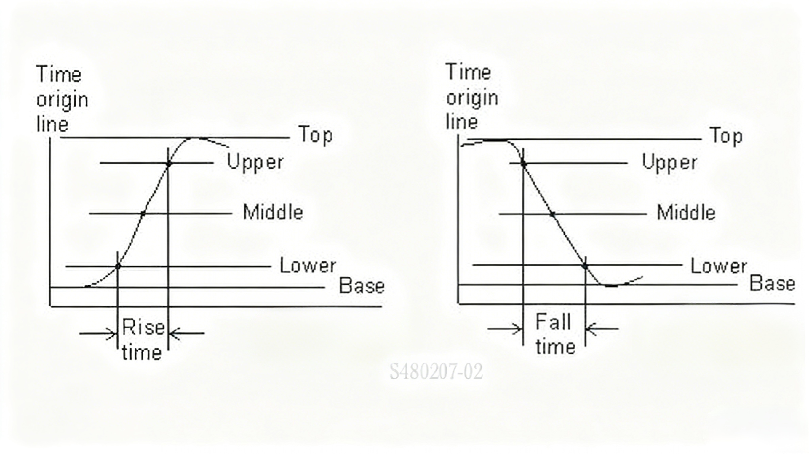
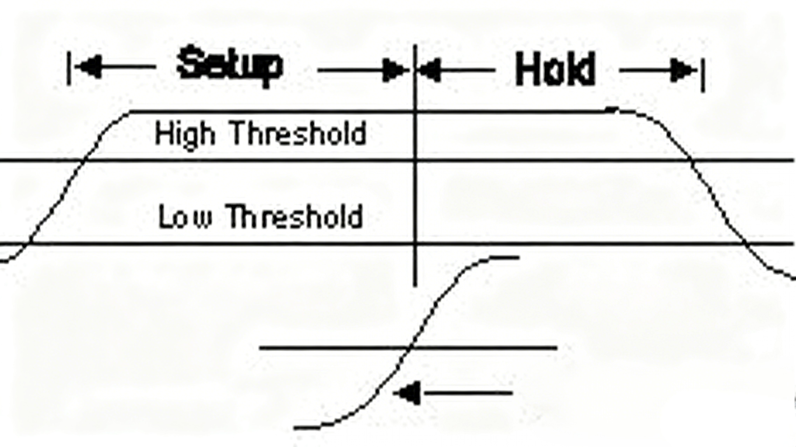
Rise Time: The rise time is the time on the upper threshold minus the time on the lower threshold of the edge you are measuring. The fall time is similar, i.e., the time on the lower threshold minus the time on the upper threshold of the edge you are measuring.
Pulse Width: The pulse width is the time from the middle threshold of the first rising edge to the middle threshold of the next falling edge.
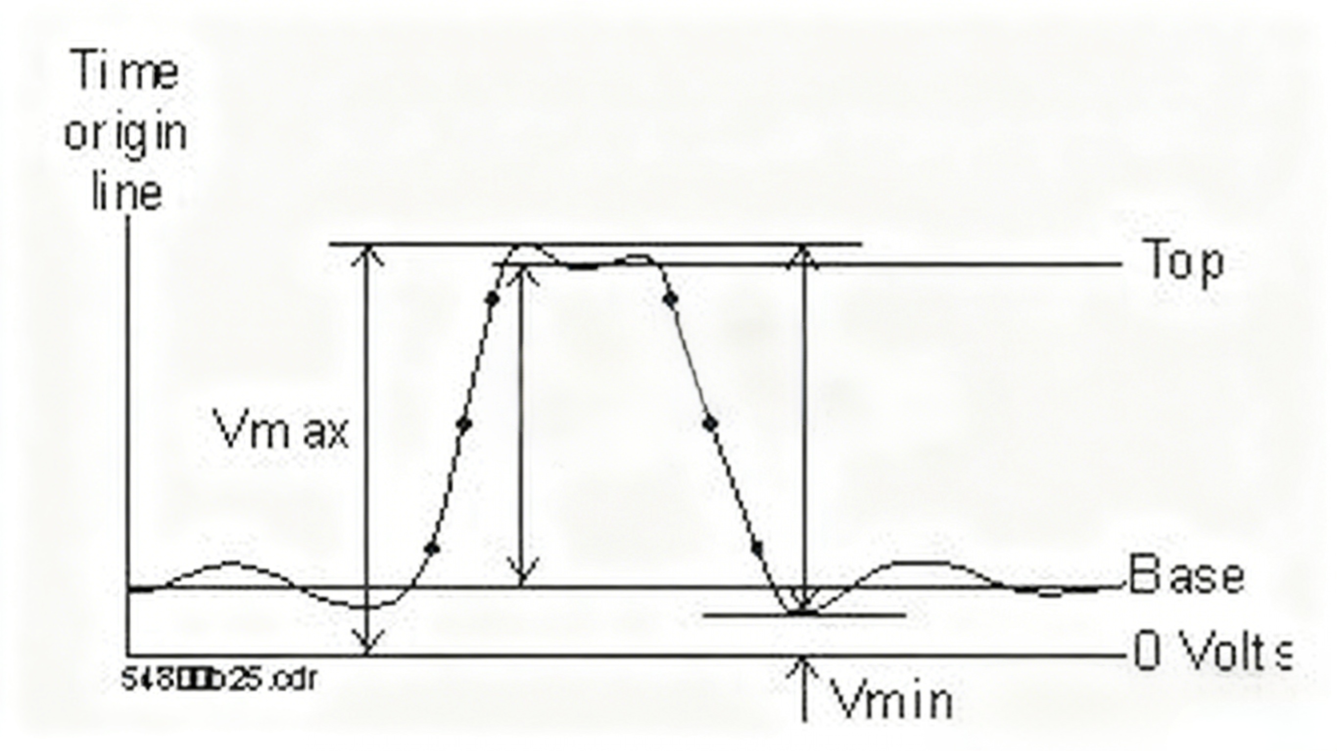
Amplitude and other voltage measurements: This is a measurement of the amplitude of the waveform display. Typically, you can also measure Peak to Peak Voltage, Maximum Voltage, Minimum Voltage, and Average Voltage.
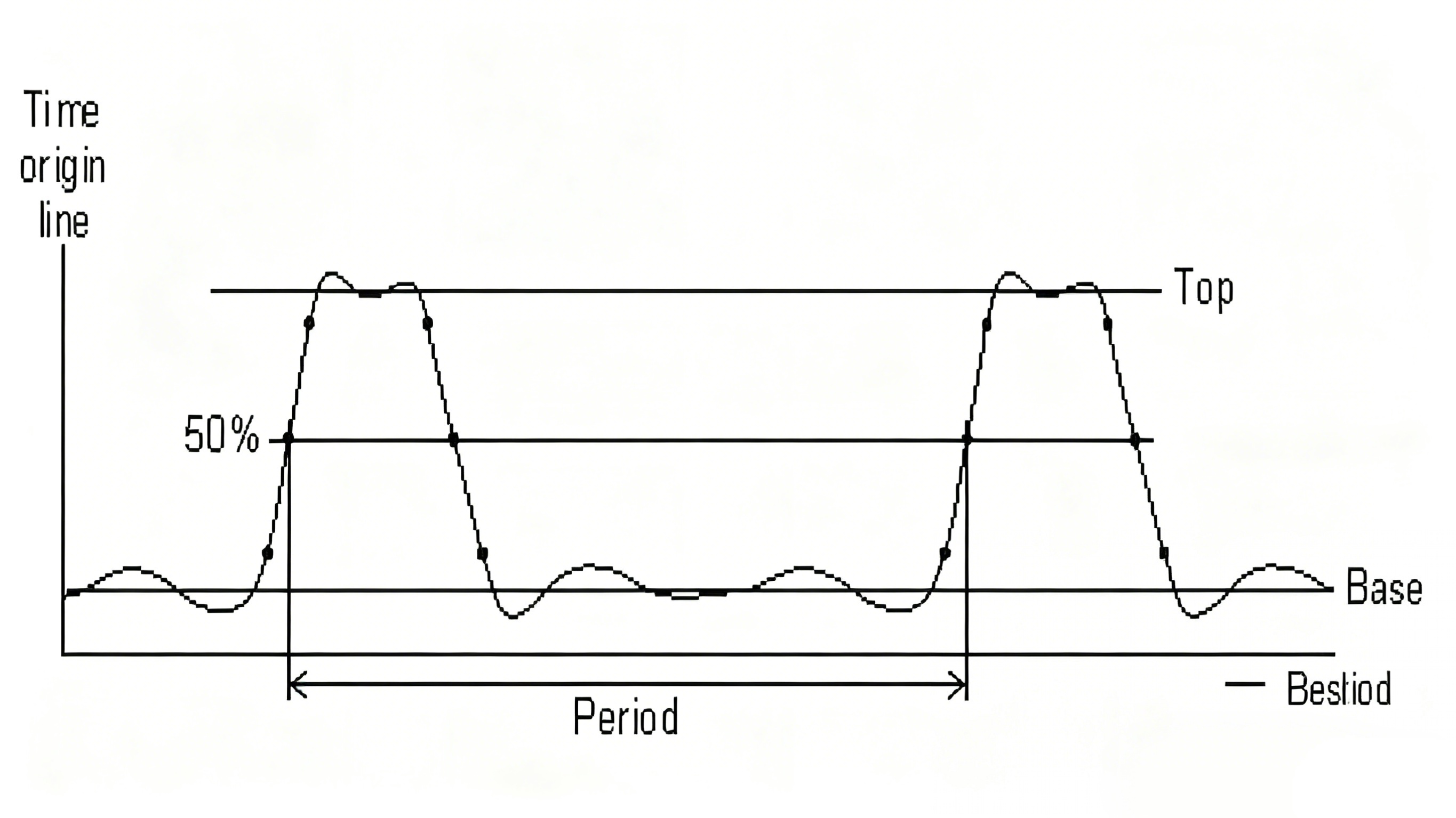
Period / Frequency: The period is defined as the time between two consecutive crossing point voltages at the center threshold. Frequency is defined as 1/period.
Establishment and Hold Time: The establishment time is the minimum amount of time that the data needs to remain stable before the clock touch arrives. The hold time is the minimum amount of time that the data needs to remain stable after the clock trigger event arrives.
Eye Diagram: An eye diagram is simply a series of pulses (000,001,010,011, 100, 101,110,111) received at the receiving end that are simultaneously superimposed on a high-speed oscilloscope to form an eye diagram. With the addition of an eye diagram template, signals can be quickly evaluated to see if they meet bus requirements or system requirements.
There are many other measurements on the oscilloscope, such as duty cycle, offset, noise, jitter, and other parameters. Here are just a few basic measurement concepts.
Traditionally, oscilloscopes measure parameters in the time domain. However, with the development of technology, oscilloscopes have diversified, allowing some to also measure parameters in the frequency domain.
This is particularly useful in power supply integrity and EMC analysis, where the data is often converted into a time domain signal frequency domain curve for analysis. Observe what frequency band problems, and then "the right medicine" to solve the problem.
5.3 Power Supply Test
(1) ripple and noise test
Switching power supply ripple refers to the superimposed ripple on the output voltage of the switching power supply, with a frequency and switching frequency consistent with the amount of AC generated by the current ripple of the switching power supply, as influenced by the capacitor's ESR. Noise is generally referred to as the full bandwidth of the output voltage superimposed on the AC quantity.
When measuring ripple and noise, you need to use the isolator + coaxial cable, and the capacitance of the isolator needs to be determined according to the switching frequency.
Ripple measurement: Use a coaxial cable to lead the output from the power module to the spacer, and then connect to the oscilloscope through the coaxial cable. Oscilloscope settings include 50 ohms of impedance, AC coupling, and a bandwidth limited to 20MHz, followed by measurements and readings. The measured waveform generally approximates a triangular waveform.
Noise measurement: Cancel the bandwidth limit of the oscilloscope, and then carry out measurements and readings with the rest of the configuration unchanged.
(2) Power loop test
In reality, the feedback loop often plays a role in stabilizing the static operating point of the circuit, so we can not simply disconnect the loop to measure the loop gain. After the feedback loop is disconnected, the circuit is saturated directly at the output because of input misalignment, etc., and no meaningful measurements can be made in this case.
To overcome this problem, we must make measurements with the loop closed, and one possible means of doing this is loop injection. The figure below illustrates a typical loop injection method. To minimize error, we have special requirements for selecting the injection point, typically ensuring that the impedance looking in at one end is significantly greater than the impedance looking in at the other end. A preferred injection point is between the outputs and the feedback network, and other injection points, such as between the error amplifier and the power transistor, are also feasible.
To maintain a closed loop, we insert a tiny resistor at the injection point, allowing the injected signal to enter the loop without breaking it. The value of this injection resistor should be small enough, usually much less than the equivalent impedance of the feedback network, to ensure that the effect of the injection resistor on the feedback loop is negligible. Picotest recommends using an injection resistor of 4.99 Ω when using a J2100A transformer or the Siglent SAG1021I directly. Alternatively, an appropriately large injection resistor is also possible. Of course, a larger injection resistor is also possible.
On the other hand, since the injection resistor is connected in parallel with the injection transformer, a smaller injection resistor reduces the lower frequency limit of the transformer's operation, which is useful when very low frequencies are to be measured. In principle, the injection of the signal must not affect the static operating point of the loop.
To solve the problem of a common ground between the signal source and the DUT in real circuits, it is often necessary to use an injection transformer. Alternatively, you can directly use a signal source with isolation.
6. Getting Started
6.1 Basic operation: connections, probes & measurement flow
(1) Step 1. Check packing items
① Check the shipping carton for damage. Retain damaged shipping cartons or cushioning materials until you have checked the integrity of the contents and the mechanical and electrical properties of the oscilloscope.
② Verify that the following items are not present in the oscilloscope packaging:
- Oscilloscope.
- Power cord.
- N2841A 10:1 10 MΩ passive probe, Qty = 2.
- Documentation CD.
- Front panel labeling (if a non-English language option is selected).
③ Check the oscilloscope.
(2) Step 2. Turn on the oscilloscope power
The following steps (powering on the oscilloscope, loading default settings, and inputting waveforms) will provide a quick function check to verify that the oscilloscope is working correctly.
① Connect the power cord to the power supply. Use only the power cord designed for the oscilloscope. Use a power supply that provides the required amount of power.
The table shows the power requirements
Table1: Power Rating
|
Name
|
Typical Value
|
|
Power Rating
|
Maximum power is 50 W
100 - 120 V/50/60/400 Hz, ±10%
100 - 240 V/50/60 Hz, ±10%
|
Warning: To avoid electric shock, make sure the oscilloscope is adequately grounded.
The table shows the environmental characteristics
Table 2: Environmental Conditions
|
Name
|
Typical Value
|
|
Ambient Temperature
|
Operating: 0 °C to +50 °C
Non - operating: - 20 °C to +60 °C
|
|
Humidity
|
Operating: 80% RH at +40 °C for 24 consecutive hours (no condensation)
Non - operating: 60% RH at +60 °C for 24 consecutive hours (no condensation)
|
|
Altitude
|
Operating: 3,000 meters (9,842 feet)
Non - operating: 15,000 meters (49,213 feet)
|
|
Vibration
|
Keysight Classification GP and MIL - PRF - 28800F; Class 3 random vibration
|
|
Shock
|
Keysight Classification GP and MIL - PRF - 28800F; (30 grams during operation, half - sine, duration 11 milliseconds, 3 shocks per axis along the main axis direction. Total of 18 shocks)
|
|
Pollution Degree 2
|
Generally only produces dry, non - conductive pollution.
Temporary conductivity due to condensation must be expected.
|
|
Indoor Use
|
For indoor use only.
|
② Turn on the oscilloscope's power supply.
(3) Step 3. Load Default Oscilloscope Settings
You can load the factory default settings at any time to restore the oscilloscope to its original settings.
① Press the Default Setup [Default Setup] key on the front panel.
② While the Default menu is displayed, press Menu On/Off to close the menu. (You can use the Undo softkey in the Default menu to cancel the default setting and return to the previous setting.
(4) Step 4. Inputting Waveforms
Input the waveform into the channel of the oscilloscope. Input the probe compensation signal from the front panel of the oscilloscope using one of the supplied passive probes.
To avoid damaging the oscilloscope, make sure that the input voltage on the BNC connector does not exceed the maximum voltage (maximum 300 Vrms).
When measuring voltages above 30 V, use a 10:1 probe.
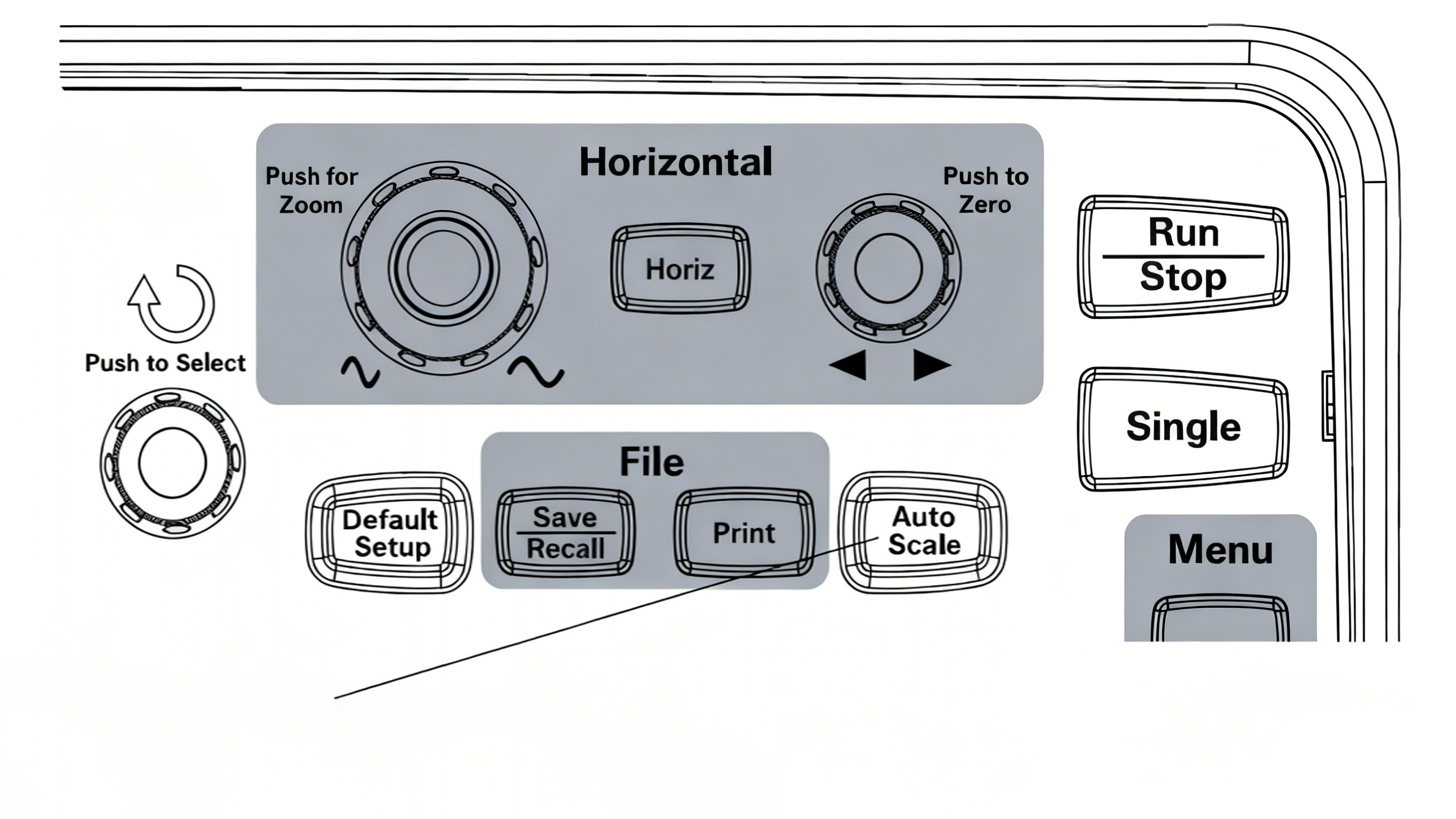
(5) Step 5. Using Auto Setup
The oscilloscope has an auto setup function that automatically sets the oscilloscope controls for the input waveform present.
Auto setup requires a waveform with a frequency greater than or equal to 50 Hz and a duty cycle greater than 1%.
① Press the [Auto Scale] key on the front panel.
② While the Auto menu is displayed, press Menu On/Off to close the menu.
The oscilloscope will open all the channels to which the waveform has been applied and set the vertical and horizontal scales accordingly. It also selects the time base range according to the trigger source. The trigger source chosen is the highest numbered channel to which the waveform has been applied.
(You can use the Undo softkey in the Auto menu to cancel the automatic setting and return to the previous setting.)
The oscilloscope has been configured for the following default control settings:
Table for Auto Setup Default Settings
|
Menu
|
Settings
|
|
Horizontal Time Base
|
Y - T (Amplitude vs. Time)
|
|
Acquisition Mode
|
Standard
|
|
Vertical Coupling
|
Adjust to AC or DC according to the waveform.
|
|
Vertical "V/div"
|
Adjust
|
|
Volts/Div
|
Coarse Adjust
|
|
Bandwidth Limit
|
Off
|
|
Waveform Inversion
|
Off
|
|
Horizontal Position
|
Relative to Center
|
|
Horizontal "s/div"
|
Adjust
|
|
Trigger Type
|
Edge
|
|
Trigger Source
|
Automatically measure the channel with input waveform.
|
|
Trigger Voltage
|
Mid - point Setting
|
|
Trigger Mode
|
Auto
|
|
Trigger Coupling
|
DC
|
(6) Step 6. Compensate Probe
Compensate the Probe to match the input channel. The Probe should be compensated whenever the Probe is connected to the input channel for the first time.
Oscilloscope Low Frequency Compensation
For the supplied passive Probe:
① Set the " Probe" menu attenuation to 10X. If using a probe hook tip, securely insert the hook tip into the Probe to ensure proper connection.
② Connect the probe tip to the Probe Compensation connector and connect the ground lead to the Probe Compensator ground connector.
③ Press the Auto Setup [Auto Scale] front panel key.
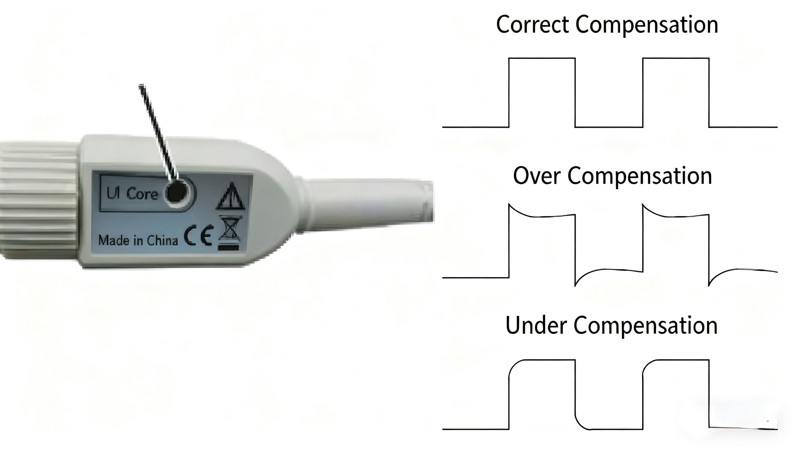
④ If the waveform does not look like the correctly compensated waveform shown in Figure 4, use a non-metallic tool to adjust the Low Frequency Compensation Adjustment on the Probe to obtain as flat a square wave as possible.
Oscilloscope Low-Frequency Compensation Adjustment
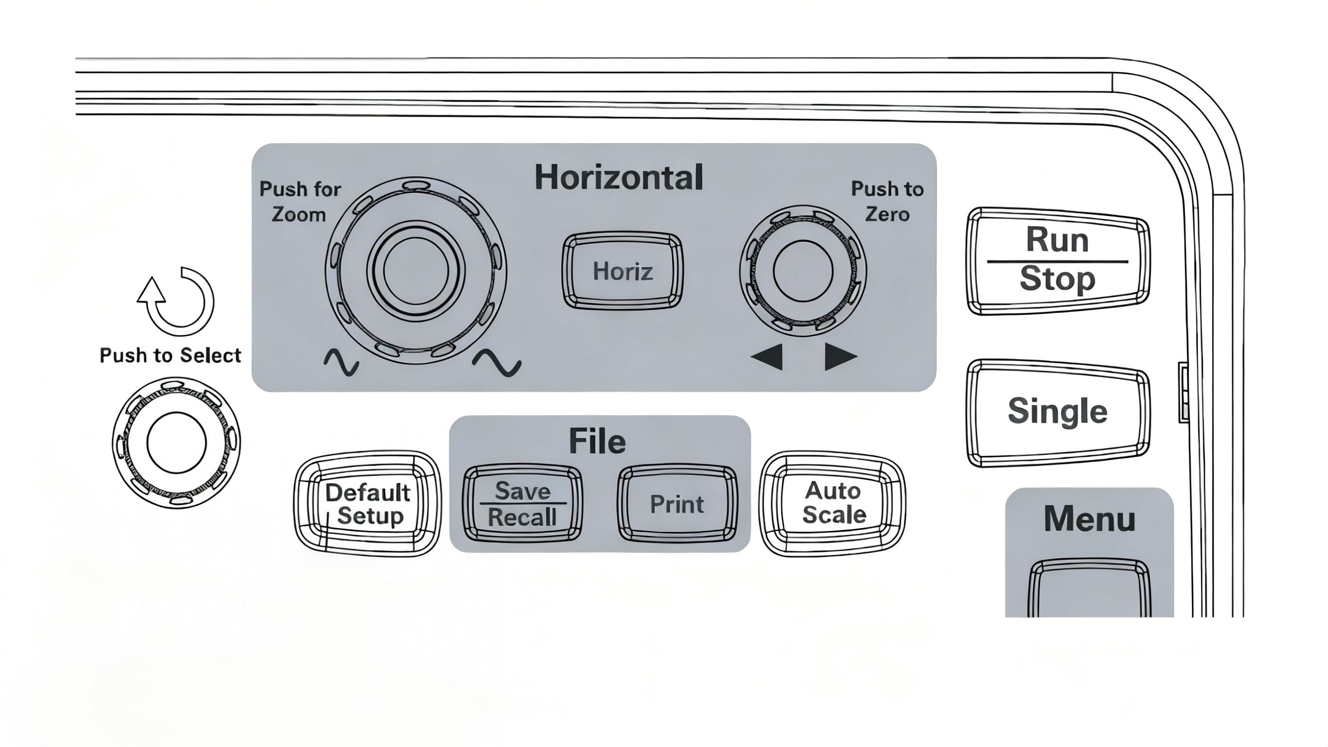
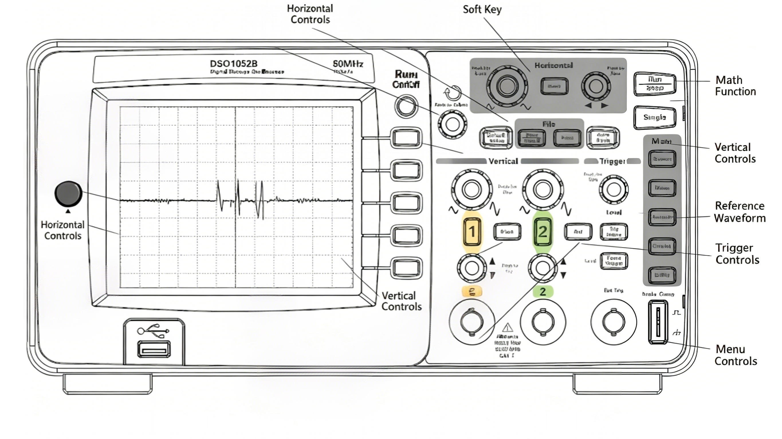
(7) Step 7. Familiarize Yourself with the Oscilloscope Front Panel Controls
Before using the oscilloscope, you should familiarize yourself with the front panel controls.
The front panel has knobs, keys, and softkeys. The knobs are most often used to make adjustments. Use the keys to run the controls and change other oscilloscope settings through the menus and softkeys.
The oscilloscope front panel knobs, keys, and softkeys are defined below:
Oscilloscope Front Panel Controls
|
Controls
|
Include the following knobs and keys
|
|
Input Knob
|
Used to adjust defined controls.
|
|
Setup Controls
|
Front - panel keys for Auto Scale and Default Setup.
|
|
File Controls
|
Front - panel keys for Save/Recall and Print.
|
|
Horizontal Controls
|
Position knob, front - panel key for Horiz, and adjustment knob.
|
|
Run Controls
|
Front - panel keys for Run/Stop and Single.
|
|
Menu Controls
|
Front - panel keys for Cursors, Meas, Acquire, Display, and Utility.
|
|
Trigger Controls
|
Level knob, front - panel key for Menu, and front - panel key for Force Trigger.
|
|
Vertical Controls
|
Vertical position knob, vertical adjustment knob, channels (such as [1], [2], etc.), front - panel keys for Math and Ref.
|
|
Soft Keys
|
There are five gray keys from top to bottom on the right side of the screen, which can select adjacent menu items in the currently displayed menu.
|
Definitions of Oscilloscope Front Panel Knobs, Keys, and Softkeys
Front Panel Labeling in Different Languages
If the Language other than English option is selected, a front panel decal is available for the selected Language.
To install the front panel decal
① Insert the tab on the left side of the sticker into the appropriate slot on the front panel.
② Gently press the sticker onto the knobs and buttons.
③ When the decal is aligned with the front panel, insert the tab on the right side of the decal into the slot on the front panel. 4 Spread the decal flat. It should be fixed on the front panel.
(8) Step 8. Familiarizing Yourself with the Oscilloscope Display
Using the Oscilloscope Softkey Menu
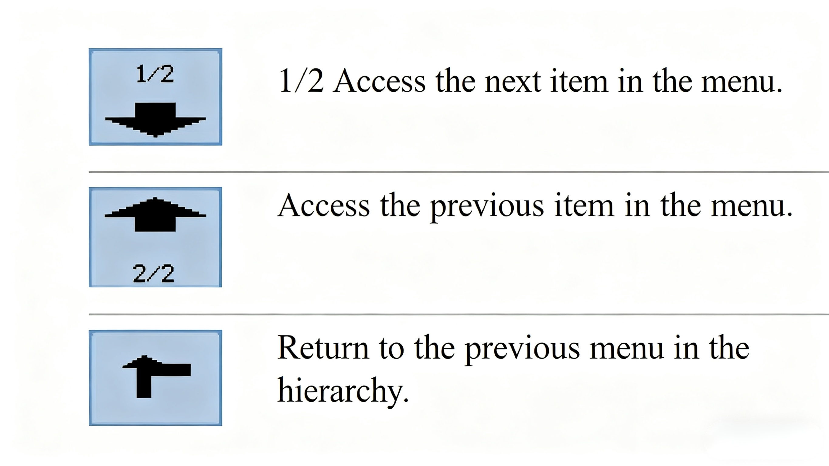
When one of the oscilloscope front panel keys opens a menu, five softkeys can be used to select items from the menu. Some commonly used menu options are listed below:
Menu On/Off [Menu On/Off] The front panel keys close the menu or open the last accessed menu again.
Use the Menu Hold item in the Display menu to select how long the menu is displayed.
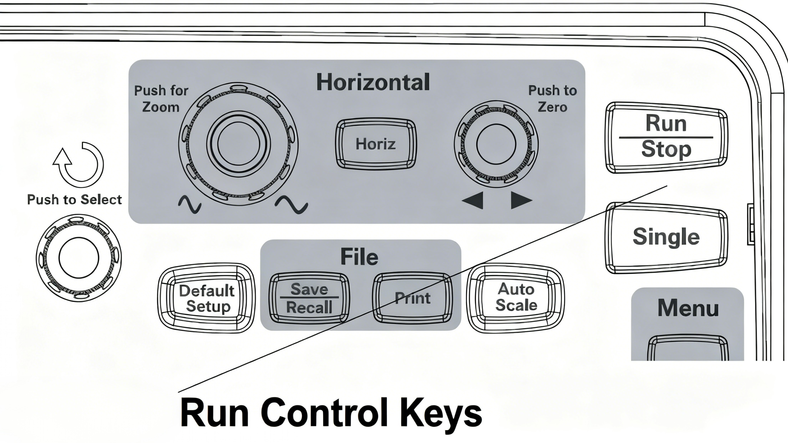
(9) Step 9. Using the Run Control Keys
There are two front panel keys for starting and stopping the oscilloscope acquisition system: Run/Stop and Single.
When the Run/Stop key is green, the oscilloscope is acquiring data. To stop data acquisition, press Run/Stop. After stopping, the last acquired waveform will be displayed.
When the Run/Stop [Run/Stop] key is red, data acquisition has stopped. To start data acquisition, press the Run/Stop [Run/Stop].
To capture and display a single acquisition (regardless of whether the oscilloscope is running or stopped), press the Single [Single] key.
[Single]. After a single acquisition has been captured and displayed, the Run/Stop key is red.
(10) Step 10. Accessing the Built-in Help
The oscilloscope has built-in quick help information. To access the built-in help:
Press and hold the front panel keys, softkeys, and pushable knobs for which you want to access their quick help information. The built-in help is available in 11 different languages.
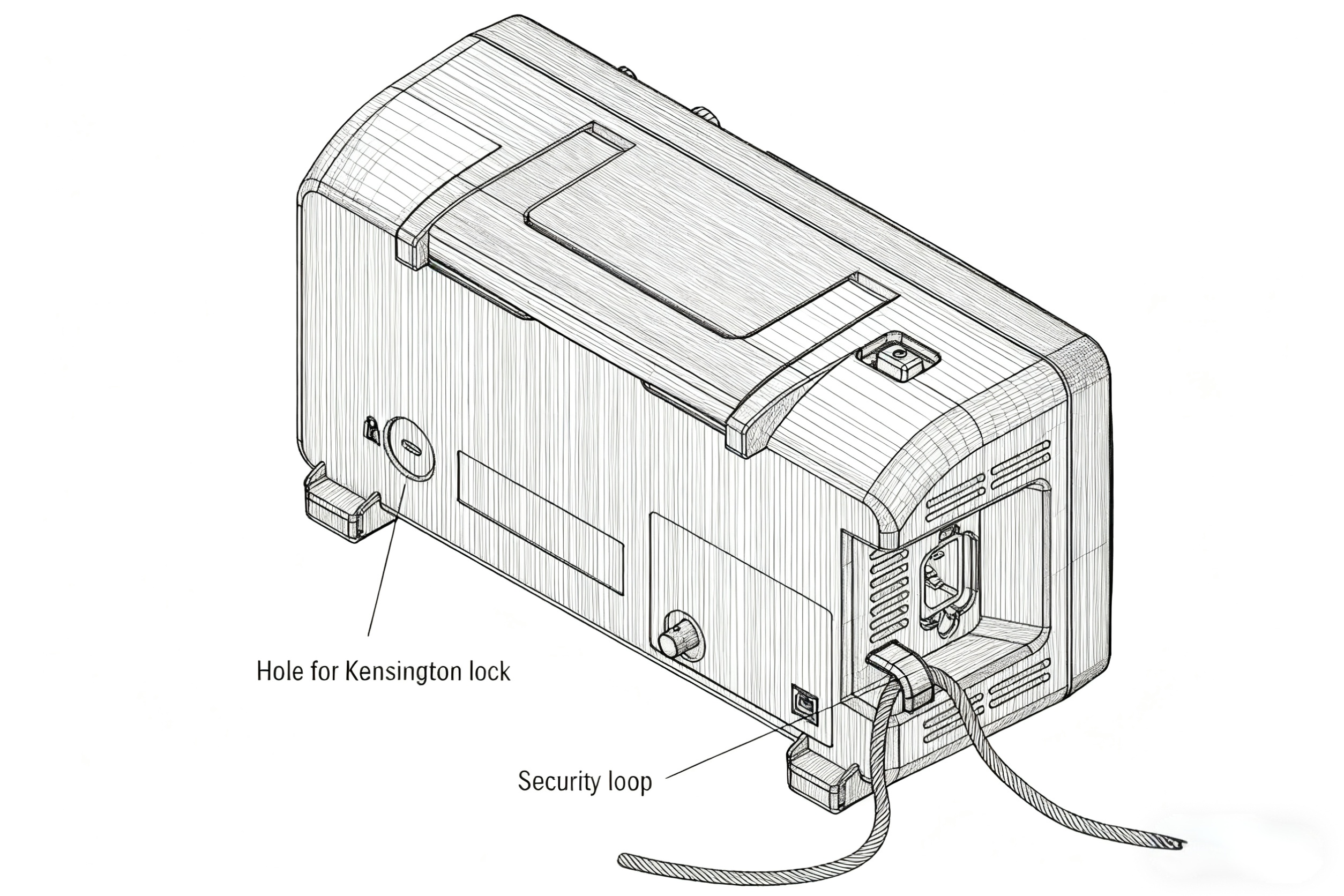
(11) Step 11. Fixed Oscilloscopes
To secure the 1000B Series oscilloscopes in place, use the anti-theft locking holes or safety rings.
6.2 Troubleshooting examples (step-by-step with screenshots)
Ideally, all probes should be a wire that does not cause any interference with the device under test and, when connected to your circuit, has an infinite input resistance, zero capacitance, and zero inductance. This will accurately replicate the signal under test. The reality, however, is that the Probe introduces a loading effect into the circuit. Resistive, capacitive, and inductive components on the Probe may alter the response of the circuit under test.
Learn about the errors that can be encountered in testing and how measurements can be improved through better operation. The electrical characteristics of the Probe can affect the measurement results and the operation of the circuit. Taking steps to ensure that these effects are within acceptable limits is a critical step for successful measurements. The following are seven common errors when using an oscilloscope:
(1) Error 1: Failure to calibrate the Probe
Probes are calibrated after they leave the factory, but they are not calibrated for the oscilloscope front end. If they are not calibrated on the oscilloscope input, then correct measurements cannot be obtained.
Active Probes
If active probes are not calibrated for the oscilloscope, you will see differences in vertical voltage measurements and rising edge timing (and possibly some distortion) during testing. Most oscilloscopes have a reference or auxiliary output and an operating guide to guide the engineer through the calibration of the Probe.
The figure above shows the 50 MHz signal input to the oscilloscope from the SMA cable and adapter on channel 1 (yellow trace). The green trace is the same signal input to the oscilloscope via the active Probe on Channel 2. Note that the generator output on Channel 1 is 1.04 Vpp (volts peak-to-peak) and the signal detected on Channel 2 is 965 mV (millivolts). Also, the offset between channel one and channel 2 is up to 3 ms (milliseconds), so the rise times cannot be lined up at all.
Passive Probes
The variable capacitance of the Probe can be adjusted to match the compensation to the oscilloscope input being used ideally. Most oscilloscopes have a square wave output that can be used for calibration or reference. Probe this connection and check that the waveform is square. Adjust the variable capacitance as necessary to eliminate any downshoot or overshoot.
If this Probe is calibrated, the results will be much improved. The results after proper amplitude and offset calibration can be seen in the graph. The amplitude is now enhanced to 972 mVpp, the offset is corrected, and the two rise times remain consistent.
(2) Error 2: Increased Probe Load Effect
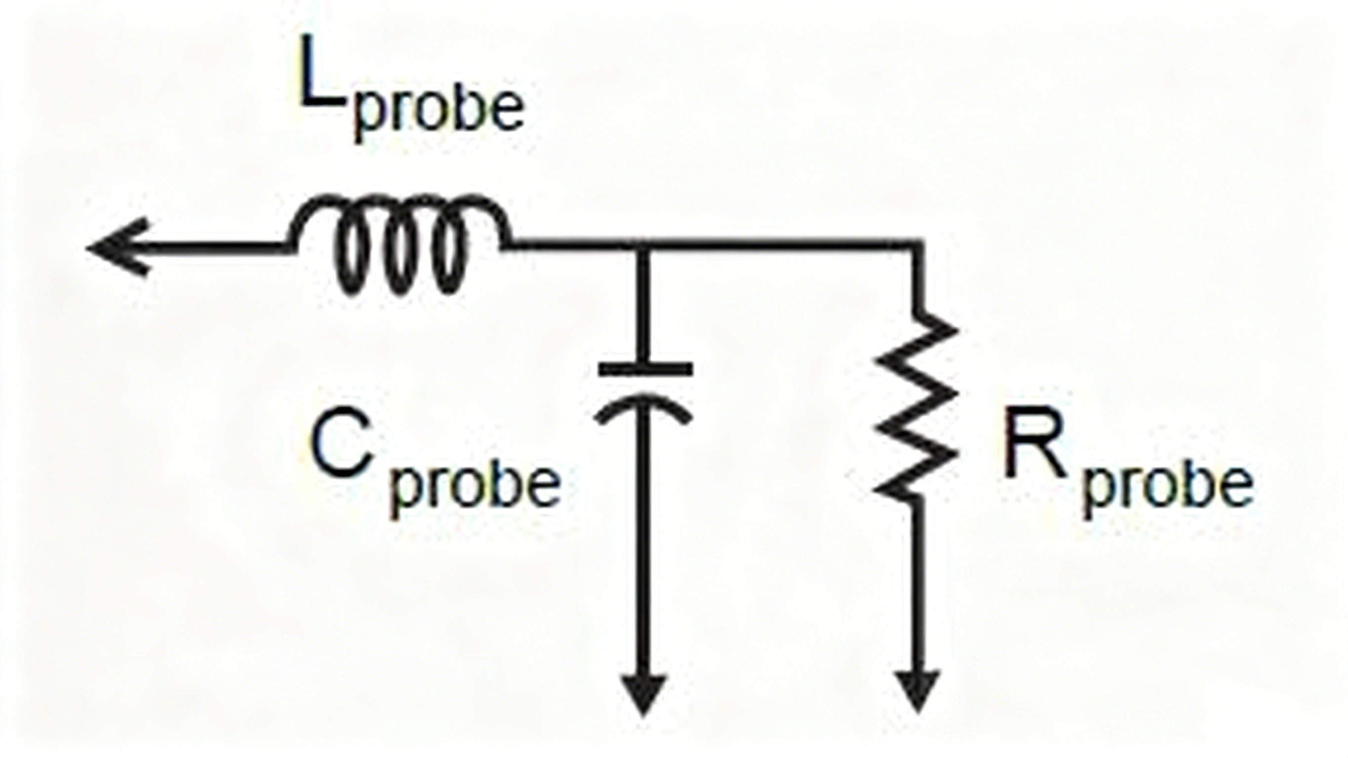
As soon as a probe is connected to an oscilloscope and it is brought into contact with the device to be measured, the Probe becomes part of the circuit. The resistive, capacitive, and inductive load effects that the Probe applies to the device under test can affect the signal that the engineer sees on the oscilloscope screen. These load effects may change the operating state of the circuit under test. Understanding these load effects helps engineers avoid selecting the wrong Probe for a particular circuit or system. Probes have resistance, capacitance, and inductance characteristics as shown in the figure.
It may be necessary to find ways to add long leads or wires to reach probes where the surroundings are too tight. However, adding attachments or probes to a probe can reduce bandwidth, increase loading effects, and consequently cause the frequency response to no longer be flat.
Use the shortest possible leads to maintain the bandwidth and accuracy of the Probe. Typically, the longer the input wire or leads to the Probe, the more the bandwidth is reduced. Narrower bandwidth measurements may not be affected as much. However, when making wider bandwidth measurements, especially above 1 GHz, you need to be careful in choosing the probes and accessories you use. As the probe bandwidth decreases, you lose the ability to measure fast rise times.
It is also a good idea to use shorter ground leads because the longer they are, the more inductance they introduce. Keep ground leads as brief as possible and as close to the system ground point as possible to ensure repeatable and accurate measurements.
Tip: If you must add wire to the Probe to reach a hard-to-reach probe point, it is a good idea to add a resistor to the Probe to dampen the resonance caused by the added wire. You may not be able to solve the bandwidth limitation problem when adding long leads, but you can flatten the frequency response. To determine the size of the resistor to be used, probe a known square wave, such as the reference square wave provided on the oscilloscope. If the resistor is set correctly, you will see a clean square wave (except that its bandwidth may be limited). If the signal is ringing, increase the size of the resistor. Single-ended probes require only one additional resistor at the Probe. If you are using a differential probe, add a resistor to each lead.
(3) Error 3: Not Utilizing Your Differential Probe to Its Fullest Potential
Many people think that they only use differential probes when probing differential signals. Is it possible to use differential probes when probing single-ended signals? Yes, it is. If used properly, this will save a lot of time and money in testing and improve the accuracy of your measurements. Maximize the use of differential probes to get the best signal fidelity possible.
Differential probes can make the exact measurements as single-ended probes. Because differential probes have common-mode rejection on both inputs, the noise in the differential measurement result is significantly reduced. This allows you to see a better representation of the signal from the device under test without being misled by the random noise added by the Probe.
The blue single-ended measurement signal and the red differential measurement signal are shown in the figure. The blue single-ended measurement exhibits significantly more noise than the red differential measurement, primarily due to the single-ended probe's lack of standard mode correction.
(4) Error 4: Choosing the wrong current Probe
High-current and low-current measurements do not require the same level of detail to be captured. It is up to the engineer to know which current Probe is the better choice for the application and what troubles may be encountered by using the wrong Probe.
Large Current Measurements
If a clamp-on probe is used to measure large currents (10A - 3000A), the device to be measured must be small enough for the clamp-on probe to clamp onto it. If the device is too large for the clamp-on probe to hold, the engineer may need to add extra wires to the probe clamp, which will alter the device's characteristics under test. A better approach is to use the right tool for the job.
The best solution is to use a high-current probe with a flexible loop probe tip. This flexible loop can be wrapped around any device. This Probe is called a Rogowski coil. It allows engineers to probe devices without adding components of unknown characteristics, allowing measurements to maintain a high degree of signal integrity. They also enable engineers to measure large currents from mA levels to hundreds of kA. Note that they only measure AC so that the DC component will be isolated. They are also less sensitive than some current probes. This is usually not a problem for large current measurements. But when measuring small currents, sensitivity and the ability to see the DC component become essential. Remember that what works for one measurement does not necessarily work for another.
Small Current Measurements
Dynamic range can vary greatly when measuring current from a battery-powered device. If the battery-powered device is idle or only handling a small number of background tasks, its current peaks will be small. When the device is switched to a more active state, the current peaks increase dramatically. Using an oscilloscope setup with a large vertical scale, engineers can measure large signals, but small current signals will be masked by measurement noise. On the other hand, if you use a smaller vertical scale setting, then large signals will clip, and measurements will be distorted and invalidated.
The current Probe you choose should be capable of measuring a wide range from μA to A and utilize multiple amplifiers to detect both small and large current deviations simultaneously. The two variable gain amplifiers in the Probe allow you to set up a zoomed-in view to see small current fluctuations and a zoomed-out view to see large current spikes at the same time (see figure below).
(5) Error 5: Incorrectly Handles DC Bias During Ripple and Noise Measurements
A small AC signal on a larger DC signal forms ripple and noise on a DC power supply. When the DC bias is significant, it may be necessary to use a larger voltage-per-cell setting on the oscilloscope to display the signal on the screen. This reduces the sensitivity of the measurement and increases the noise compared to a small AC signal. This means that an accurate representation of the AC portion of the signal cannot be obtained during testing.
Suppose a DC isolation capacitor is used to solve this problem. In that case, it will inevitably block some of the low-frequency AC content, preventing the engineer from observing the changes in the signal as it passes through the components on the device.
Using a power probe with a larger bias allows the waveform to be placed in the middle of the screen without removing the DC bias. This allows the entire waveform to be displayed on the screen while keeping the vertical scale small and at amplification. These settings also allow details of transients, ripple, and noise to be viewed.
(6) Error 6: Unknown Bandwidth Limits
When making essential measurements, always select a probe with sufficient bandwidth. Insufficient bandwidth can distort the signal, making it difficult for engineers to make informed engineering test or design decisions.
The generally accepted formula for bandwidth calculation is: when evaluating the rising edge from 10% to 90%, the bandwidth multiplied by the rise time equals 0.35.
BW x Tr = 0.35
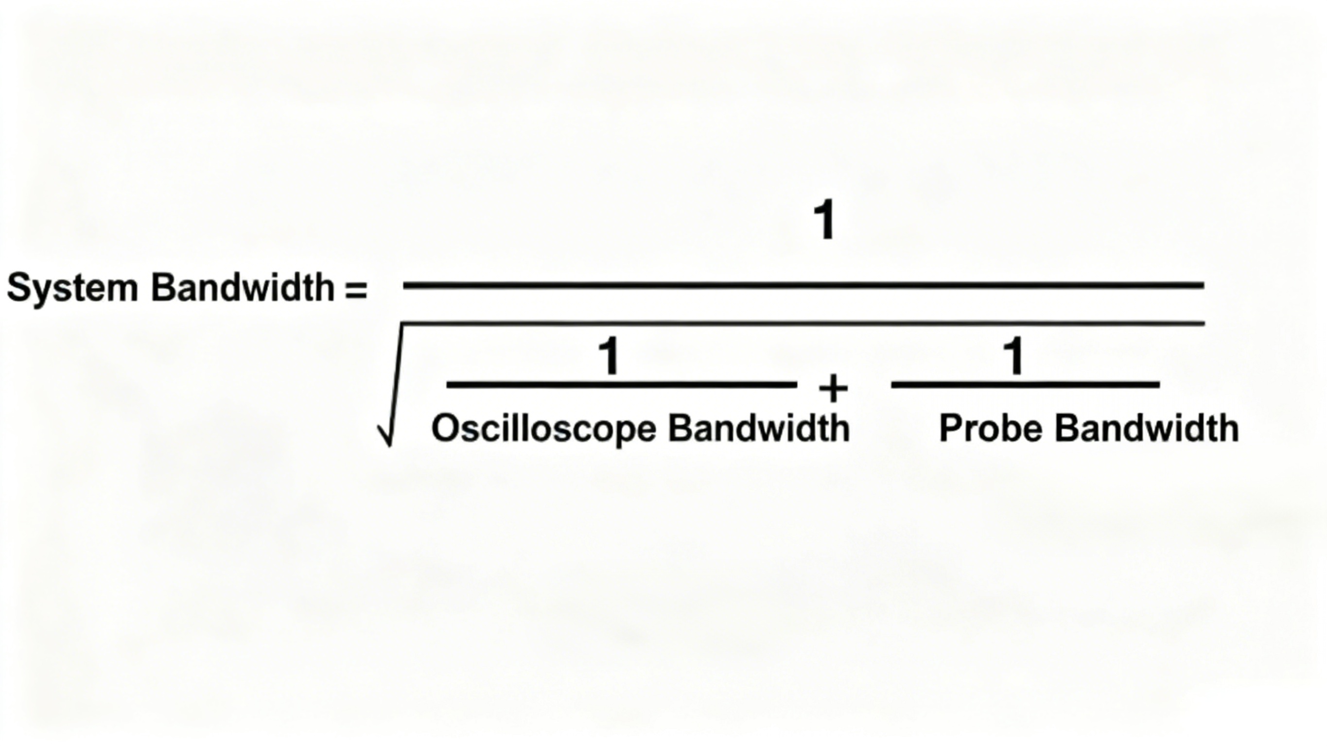
It is important to note that the overall system bandwidth is also an essential factor to consider. The bandwidth of both the Probe and the oscilloscope should be considered to determine the system bandwidth. The formula for calculating the system bandwidth is shown below.
For example, assume that the oscilloscope and probe bandwidths are both 500 MHz. Using the above formula, the system bandwidth would be 353 MHz. As can be seen, the system bandwidth is significantly reduced when compared to the two separate bandwidths of the Probe and oscilloscope.
Now, if the probe bandwidth is only 300 MHz and the oscilloscope bandwidth is still 500 MHz, then applying the above formula, the system bandwidth is further reduced to 257 MHz.
(7) Error 7: Masked Noise Effects
Probe and oscilloscope noise may cause the noise of the device under test to appear larger. Selecting a probe with the proper attenuation ratio for the engineer's application will reduce the noise added by the Probe and oscilloscope. As a result, the engineer will be able to obtain a more accurate signal and a clearer view of the device under test.
Many probe manufacturers describe probe noise as Equivalent Input Noise (EIN) and express it in Vrms. Higher attenuation ratios allow you to measure larger signals, but the downside is that the oscilloscope will detect these ratios and amplify both the signal and its noise. To see the practical results of this effect, the green trace in the figure shows the noise after amplification with a 10:1 probe.
7. Advanced features and specialized analysis
7.1 Advanced features: FFT, protocol decode, serial bus analysis
(1) FFT function
Intuitively, the time domain analysis of the oscilloscope is clearly visible, and the time domain analysis function is also the most essential function of the oscilloscope; testers are relatively familiar with the time domain analysis function. However, when further analysis of the signal is required, such as determining the proportion of harmonics and energy distribution, time domain analysis is insufficient. In this case, the utilization of oscilloscopes equipped with a Fast Fourier Transform (FFT) function to analyze the signal becomes particularly meaningful.
FFT is a potent analysis function. The digital oscilloscope has a typical application. Based on the advanced FFT analysis function, testers can accurately understand the signal introduced in the interference signal frequency, signal power spectrum, and signal frequency composition.
When the oscilloscope is switched to the FFT function, the horizontal axis is the frequency, unit (Hz); the vertical axis is the power (dB) or voltage (V). When using the FFT function of the oscilloscope, you need to pay attention to the following parameters: the number of sample points, spectral resolution, and sampling frequency.
Number of Sample Points: The number of points used to calculate the FFT.
Spectral resolution: the most minor frequency that the oscilloscope can resolve, i.e., the frequency interval between two neighboring frequency points.
Sampling frequency: the number of points collected per second.
Take the actual signal as an example. When the oscilloscope samples the digital signal, it can perform the FFT transform. Assuming that the sampling frequency is Fs, the signal frequency F, and the number of sampling points is N. The frequency of a point n is Fn. The frequency that can be resolved to Fn is related to the number of sampling points, which is calculated as follows: Fs/N, if the sampling frequency Fs is 1kHz and the number of sampling points is 1k, it can be resolved to 1Hz, that is to say, sampling the signal of 1 second and doing the FFT, the frequency resolution can be as accurate as 1Hz; if sampling 2 seconds and doing the FFT, the frequency resolution can be as precise as 1Hz; if sampling 2 seconds and doing the FFT, the frequency resolution can be as accurate as 1Hz. 1Hz; if the signal is sampled for 2 seconds and the FFT is done, the result can be precise to 0.5 Hz. If the frequency resolution is to be improved, the number of sampling points must be increased, i.e., the sampling time must be extended. Spectral resolution and sampling time are inversely related.
According to the Nyquist sampling theorem, the spectrum width after FFT can only be 1/2 of the original signal sampling rate, so the sampling frequency should be greater than 2 times the highest frequency of the signal to restore the original signal waveform. Therefore, a higher spectral resolution requires a longer sampling time, and a wider spectral distribution requires a higher sampling rate of the original signal. If we want a broader spectrum and higher resolution, the oscilloscope requires sufficient storage depth. In practice, we can follow the above method to select the appropriate oscilloscope with reference to the measured signal.
(2) Protocol decoding
Manual decoding of the serial bus according to the oscilloscope waveform display is both time-consuming and error-prone. In this relatively simple I2C signal, there may be a problem. Can you easily find the problem? Can you even tell what the signal represents? To decode this packet manually, look for the packet header, data bits, and packet tail. Confirm all data signal states (blue) against each other using the clock states (**) and convert them to hexadecimal values.
Manual decoding is compared here with the automatic decoding example. Simply defining which channels the clock and data are on and defining the thresholds for determining the logic values ("1" and "0") allows the oscilloscope to be informed of the protocol being transmitted over the bus. In a split second, the serial data can be decoded and displayed, illustrating the start, address, data, and end bits in the bus waveform display. Address and data values can be shown in hexadecimal or binary for the I2C bus.
(3) Serial bus analysis
The use of ordinary oscilloscopes can only perform general edge triggering and pulse width triggering; it is difficult to capture the complexity of the serial bus waveform. Instead, using an oscilloscope with a serial bus trigger function makes it easy to capture the desired serial data. Yokogawa's DLM2000 series digital oscilloscopes support the triggering of a variety of commonly used serial buses, including CAN/LIN/I2C/SPI/UART. They can even be triggered on user-defined non-standard serial buses. Depending on the structure of each bus, multiple trigger modes can be set. The more trigger modes, the better the ability to capture data.
In embedded systems, there are often two or even more serial bus structures at the same time. For example, in automotive electronics, CAN and LIN buses are frequently used simultaneously, and it is necessary to analyze whether the two bus communications are causing the problem. Most of the oscilloscopes with a serial bus triggering function can only trigger a bus at the same time. To achieve CAN and LIN bus triggering simultaneously, you can only use two oscilloscopes, and synchronizing the two oscilloscopes is also challenging.DLM2000 series oscilloscopes with dual-bus triggering function can be easily achieved by the combination of any two kinds of serial bus triggering.
After triggering to the desired serial data, engineers are still faced with the original waveform of the data. To efficiently analyze the bus, the waveform needs to be decoded. At present, the decoding technology used in digital oscilloscopes includes both software decoding and hardware decoding. Software decoding is the process of decoding the waveform data through the oscilloscope software operation to obtain the decoding results. Although it can reduce the cost of hardware, the CPU computing speed requirements are very high. In practical applications, software decoding oscilloscopes can decode for a few seconds or even more than ten seconds. Such decoding speed has lost the significance of real-time analysis, because most of the data has been lost in the waiting for decoding. A few high-end oscilloscopes use hardware decoding technology to solve this problem, making real-time decoding and analysis possible.
While displaying the decoding results, the decoding list of all captured frames can also be displayed, making it very easy to observe the correspondence between waveforms and decoding results.
To obtain correct decoding results, it is necessary to set the oscilloscope according to different bus parameters. Taking CAN bus analysis as an example, the following steps are required: specify the bus type as CAN, set the channel corresponding to the CAN signal, trigger the CAN bus by adjusting the trigger level and time axis, change the bit rate, set the invisible level, and so on. If it is an SPI bus, it is also necessary to specify the 3-wire or 4-wire system, the clock signal, and the chip select signal. This setup process requires careful attention; if any of these settings are incorrect, the decoding results may not be accurate. Particularly with the bit rate setting, even a slight error can lead to incorrect decoding results.
The complex setup process not only wastes part of the debugging time but also does not fully utilize the oscilloscope's role in improving development efficiency. DLM2000 oscilloscopes realize the automatic setting of serial bus trigger and decoding analysis. Users only need to set up the bus type and signal source channel; the system can automatically adjust the bit rate, trigger level, invisible level, and other settings, and in just two seconds, it can trigger waveforms and decode the results of synchronous display. This function makes the cumbersome serial bus setup very convenient and dramatically improves the development efficiency of engineers.
7.2 Calibration, probe selection & maintenance
(1) Oscilloscope Calibration
The purpose of calibration is to ensure that the measurement results of the oscilloscope conform to the manufacturer's specifications and national/international standards. It is divided into two categories: external calibration and internal self-calibration.
①External calibration
Performed by a certified metrology laboratory or manufacturer's service engineer using a calibrator (e.g., Fluke 5500A, 9500, etc.) that is 3-10 times more accurate than the oscilloscope under test. This is a legally valid, traceable calibration.
Periodicity: Usually once a year. The exact periodicity depends on laboratory requirements, usage environment, and frequency of use.
Procedure: The calibration engineer will: check the appearance and basic functions. Connect the high-precision calibrator to each channel of the oscilloscope. Test and adjust a series of key parameters, such as:
Vertical Amplitude Accuracy (Voltage Measurement): Input a standard voltage square wave to verify that the displayed voltage value is accurate.
Horizontal Time Base Accuracy (Time Measurement): Input a standard frequency signal to verify that the time base and measurement values are accurate.
Rise Time: Input a swift edge signal to verify the bandwidth and response of the oscilloscope.
Trigger Sensitivity: Verify if the trigger is stable and reliable under different settings.
Upon completion, a detailed calibration certificate will be issued, containing test data, uncertainty, and a passing conclusion.
② Internal self-calibration
This is an operation that can and should be performed periodically by the user themselves. It is not a traceable calibration, but utilizes a highly stable reference source inside the oscilloscope to compensate for errors due to temperature changes and circuit drift.
Periodicity: When the ambient temperature changes more than 5°C. After the first installation or after a long period of non-use. Monthly or quarterly as preventive maintenance.
How to operate:
Warm up the oscilloscope for 20-30 minutes to allow it to reach a stable operating temperature.
Disconnect all probe and input wires and leave the channel inputs open.
Find the "Self Calibration" or "Signal Path Compensation" function in the utility/maintenance menu of the oscilloscope.
Follow the on-screen instructions (usually just click "Start").
Do not touch or move the oscilloscope during the process.
Probe Compensation Calibration: This is a specific calibration for passive probes and is described in detail below.
(2) Probe Selection
Choosing the wrong probe can seriously degrade the performance of the oscilloscope and make an expensive oscilloscope pointless. The probe is part of the measurement system.
① Probe Types
Passive probe:
The most common are usually included with the oscilloscope. It consists of resistors and capacitors internally, with no active components.
Advantages: rugged, inexpensive, extensive dynamic range, no need for a power supply.
Disadvantages: low bandwidth (usually <500MHz), significant load effect.
Suitable for general-purpose low-speed measurements, including digital circuits, power supplies, and audio applications.
Active probes:
Contains active amplifier circuitry internally and requires a power supply (usually from an oscilloscope or external power supply).
Advantages: very high bandwidth (up to several GHz to tens of GHz), minimal load effect (input capacitance can be as low as below 1pF).
Disadvantages: expensive, low dynamic range, easily damaged (overvoltage).
Suitable for: high frequency signals, high speed digital signals (e.g., DDR, PCIe), low power circuits.
Differential Probes:
Measures the voltage difference between two test points, not the voltage to ground.
Advantages: floating ground measurement, strong noise immunity, safe measurement of high voltage differential signals.
Suitable for: switching power supplies, motor drives, three-phase circuits, bus signals (e.g., CAN, RS485).
Current probes:
Measures current (AC or AC/DC) by sensing the magnetic field around a wire.
Applicable: power supply, power consumption analysis, motor current, and inverter analysis.
②Select key parameters
Bandwidth: The combined bandwidth of the probe and oscilloscope is determined by the lower of the two. The selected probe bandwidth should be at least 3-5 times the highest frequency component of the signal under test.
Load effect: When the probe is connected to the circuit, it becomes a load and affects the circuit under test. The key parameters are input resistance and input capacitance. The input resistance should be as significant as possible (usually 1MΩ or 10MΩ) to minimize the load on the DC circuit. Input capacitance is a killer for high-frequency measurements. The smaller the capacitance, the less effect it will have on the edges of high-speed signals. Herein lies the advantage of active probes.
Attenuation Ratio: Commonly available are 1X, 10X, 100X, etc. A 10X probe allows for higher voltage measurements, but also attenuates the signal to 1/10th, potentially degrading the signal-to-noise ratio for small signal measurements.
Voltage range: Ensure the maximum input voltage of the probe (including both DC and AC peaks) is significantly higher than the signal under test, particularly when measuring power supplies or power circuits.
(3) Probe and Oscilloscope Maintenance
Good maintenance habits can extend the life of the equipment and ensure measurement accuracy.
① Daily use and maintenance
Mechanical protection: Avoid dropping and hitting the probe and oscilloscope. Align the slots when connecting and do not use excessive force. Do not pull, bend, or crush the probe cable. The arc should be as large as possible when winding.
Electrical protection: Never exceed the maximum input voltage. Pay particular attention to the very fragile nature of active probes. When measuring unfamiliar circuits, use the 10X attenuation mode first and start at a higher voltage level. When measuring high voltages (e.g., mains), always use high voltage differential probes and pay attention to safety regulations.
Environmental protection: Keep the probe connector and oscilloscope interface clean and dry. Avoid dust and liquid intrusion. Store in a dry, temperature-suitable environment and avoid direct sunlight.
② Probe Compensation Calibration
This is an operation that the user must check every time before using the passive probe. Incorrect compensation will result in wrong amplitude and rise time measurement.
Steps:
Connect the probe to one channel of the oscilloscope (set to 10X attenuation).
Hook the probe tip to the square wave reference output of the oscilloscope (usually a 1kHz, 5V or 2.5V square wave signal).
Using the adjustment tool that comes with the probe (usually a non-inductive screwdriver), adjust the compensation capacitor adjustment hole on the probe body.
Observe the waveform to make a perfect square wave.
Overcompensation: The waveform edges become overshoot and rounded.
Undercompensation: Waveform edges become slow and rounded.
Correctly compensated: Waveform edges are steep and flat.
Note: Each channel and each probe should be compensated separately.
8.How to choose an oscilloscope (engineer's checklist)
8.1 Key Technical Specification: Bandwidth
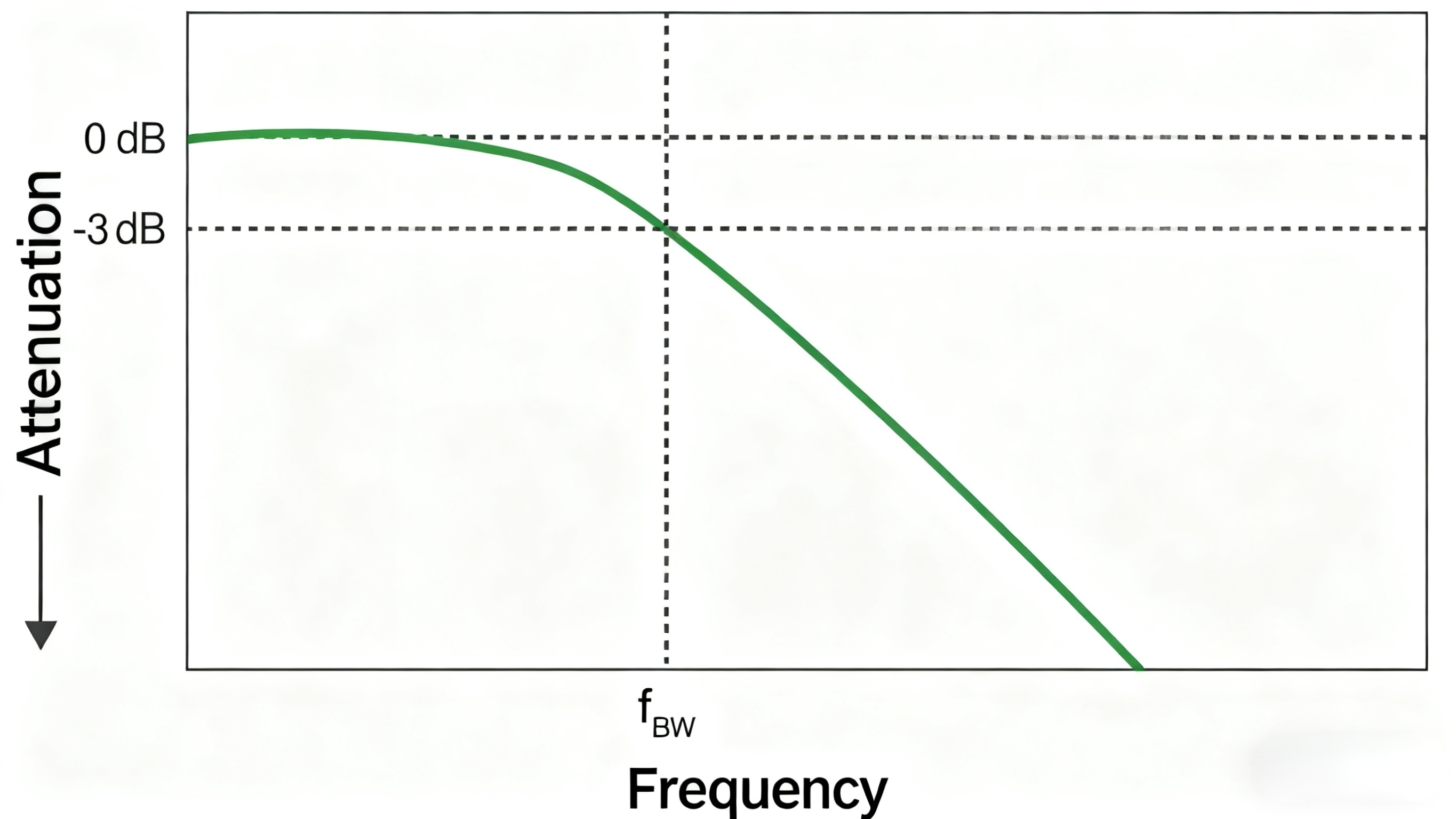
Bandwidth is the range of frequencies that an oscilloscope can measure. Oscilloscopes are one of the few broadband instruments capable of making measurements from DC (0 Hz) to their specified bandwidth. The bandwidth specification is an important consideration when purchasing an oscilloscope; if the oscilloscope does not have sufficient bandwidth, it will not be able to make accurate measurements.
The frequency response of an oscilloscope front-end amplifier is similar to that of a low-pass filter. The shape of the curve in the figure indicates that the oscilloscope is capable of measuring most of the signal components in the frequency range from DC to the 3 dB drop in signal attenuation. The oscilloscope defines the frequency corresponding to this -3 dB point as the "bandwidth" at which the voltage drops by approximately 30%.
When using an oscilloscope, you want it to capture the true rising edge of the signal accurately. The bandwidth mainly realizes this function. You can only capture a signal accurately if you have enough bandwidth. If you don't have enough bandwidth, you'll miss critical signal details and end up making flawed design assumptions.
Engineers often think that measuring a 100 MHz signal requires only 100 MHz bandwidth, but this is not the case. Our recommendation for bandwidth is to choose an oscilloscope with a bandwidth five times higher than the fastest frequency or clock rate in the device. Most oscilloscopes with bandwidths of 1 GHz and below have a Gaussian frequency response, as shown in Figure 2. This is a low-pass frequency response that decays at higher frequencies.
8.2 Sample Rate
The oscilloscope's analog-to-digital converter (ADC) is capable of converting analog signals into digital signals. This analog-to-digital conversion rate is called the "sampling rate". The manufacturer specifies the unit of sample rate as sample points/second. For example, a 300 MHz oscilloscope has a sampling rate of 2 gigasample/s. This sampling rate can also be expressed as 2 Gsample/s, 2 GaSa/s, or 2 GSp/s.
The sampling rate of the oscilloscope should be at least 2.5 times the bandwidth. For example, if the oscilloscope has a bandwidth of 1.5 GHz, the sampling rate should be higher than 3.75 Gsample/s. Most digital oscilloscopes usually meet this minimum requirement. However, oscilloscopes may interleave multiple channels to provide the maximum sampling rate.
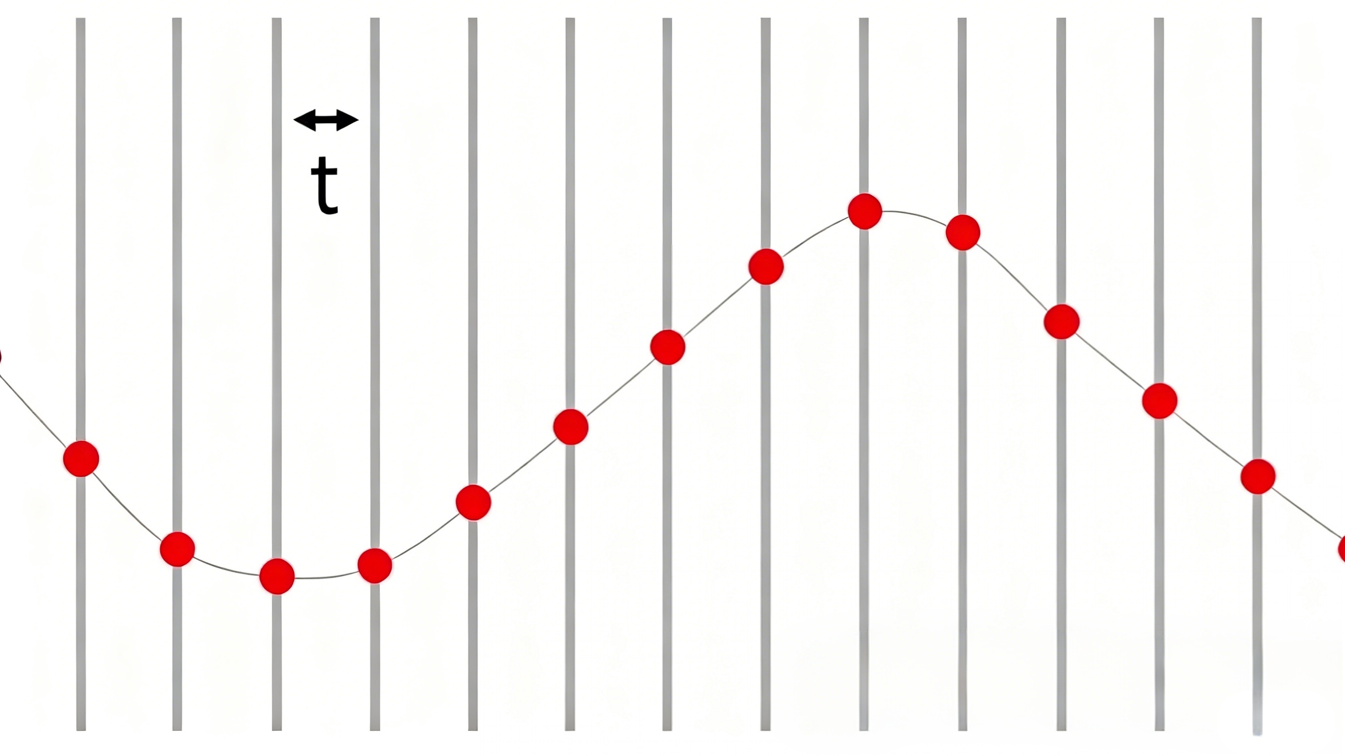
In the case of an analog-to-digital converter (ADC), which converts an analog signal to a digital signal, it collects "samples" or data points of the analog signal, which the ADC uses to reconstruct the signal on the oscilloscope screen digitally. The rate at which these samples are collected is called the sampling rate and is measured in samples per second (Sa/s). In well-designed oscilloscopes, such as the InfiniiVision family of oscilloscopes, these samples are collected at uniform time intervals.
When you see the resulting signal on the screen, you will not know these sample points, but a smooth waveform. The oscilloscope inserts traces between each collected sample. However, if not enough samples are taken, then the interpolation does not represent the signal well, resulting in incorrect measurements.
Sampling at too low a rate not only leads to distortion, but it also causes you to miss critical signal details that were not sampled, such as burrs and errors. In the figure, we can see how much signal detail is missed by a low sample rate (or "undersampling").
8.3 Fast Waveform Capture Rate is Key
The waveform capture rate is also known as the trigger rate. This indicates how fast the oscilloscope captures waveforms between trigger events. In general, the quicker the oscilloscope resets and retriggers, the shorter the dead time between acquisitions.
The dead time is the interval between acquisitions during which the oscilloscope cannot capture the waveform. The shorter the dead time and the faster the trigger rate, the greater the probability that the oscilloscope will capture episodic events such as transient pulses.
As with sampling rate, the higher the waveform capture rate of an oscilloscope, the more detail you see in the signal. If the oscilloscope's waveform capture rate is insufficient, you will not be able to detect anomalies in the signal. It's like rolling a dice. The more times you roll the dice, the higher the probability of getting a particular combination of numbers. Similarly, the more times the oscilloscope is updated, the more likely you are to capture rare events.
All oscilloscopes have a certain amount of "quiet time" or "blind time" between each capture and the display of the acquisition results.
During this time, rare signal anomalies, such as burrs, may occur. The slower the waveform capture rate, the longer the silence time, and the more signal detail you miss. Conversely, the higher the waveform capture rate, the shorter the silence time and the more real signal detail you see.
For example, an update rate of a few thousand waveforms per second may seem fast, but what if there is a burr in your signal that has a one-in-a-million chance of occurring? If the update rate is too slow, you may never see the burr. Having a high waveform capture rate (e.g., 1,000,000 waveforms/second) is critical to increasing the probability of catching rare errors, as shown in the figure.
8.4 The Role of LAN Connectivity
Connecting your oscilloscope via LAN opens up a whole new dimension of testing and saves you even more investment. No matter where you work - whether it's a teaching lab, a design studio, or a production floor - LAN connectivity makes your processes more efficient.
This network connection allows you to work anywhere, anytime, regardless of time and place. The LAN connection enables remote control via an open Internet browser, allowing multiple engineers to work with the same instrument simultaneously. This will enable students and colleagues to share equipment usage for project work from anywhere, ultimately saving budgets.
You can send remote commands to the instrument over the LAN, as well as fully control the instrument on your PC using the emulated instrument screen and hardkey controls. Because the user interface is identical to that of the actual instrument, maintaining the instrument is much easier.
The LAN connection not only makes it easier to control the instrument but also supports instrument monitoring in large laboratory environments. This is especially helpful in teaching labs where there are many students doing research with a variety of instruments. Connecting to the network has another outstanding advantage: test automation. Automated testing is standard in both R&D and manufacturing environments.TestFlow software, which is part of BenchVue, is also a compelling offline analysis and documentation tool.
8.5 Storage Depth
ADCs store their samples in a memory buffer.ADCs have sample rates of up to a gigabyte, so the storage speed must be comparable. The number of samples stored is called the "memory depth". For example, if the channel has a 10 Mpts buffer, it can store up to 10 million samples per acquisition.
There is a direct relationship between the oscilloscope's sample rate, memory depth, and acquisition time. The time base setting determines the minimum time for the oscilloscope to acquire a signal. The acquisition system balances the storage depth and sample rate to ensure that the maximum sample rate is provided at a particular time base setting. The larger the available storage, the slower (longer) the time base setting can be when maintaining a high sample rate. In general, the greater the storage depth, the better. However, some oscilloscopes are unable to maximize the use of storage depth, while others run very slowly when using larger storage depths.
How do I choose the storage depth I need?
Unlike other essential specifications for oscilloscopes, there is no simple guide to selecting the storage depth. However, if you determine the required acquisition time, you can choose the minimum storage depth required. For example, to acquire a 10-cycle 100 MHz clock signal, you need to gain at least 100 nanoseconds. An ADC with a sample rate of 1 Gsample/s samples once per nanosecond. Therefore, you need a memory depth of 100 samples.
8.6 ADC Bit Count
The analog-to-digital converter of the oscilloscope outputs binary values. Like other ADCs, the number of bits in these binary values determines the resolution of the oscilloscope ADC. For example, an 8-bit ADC can output 256 different voltage level values, a 10-bit ADC can output 1,024 types, and a 12-bit ADC can output 4,096 types.
Although ADC resolution affects the measurement accuracy of an oscilloscope, it is not the only factor to be considered. Accuracy is the difference between the expected measurement value and the actual value. In other words, precision indicates the uncertainty of a measurement. Resolution is the smallest change that the measurement system can display. In an oscilloscope, the bit width of the ADC determines the resolution. Sensitivity is the smallest change that can be detected. This definition is more similar to the resolution definition, and the individual components of an acquisition system may be very sensitive. However, overall sensitivity is related to accuracy and resolution.
8.7 Triggering
The trigger system of a digital oscilloscope observes specific events in the signal under test. The trigger system initiates a trigger operation when it detects an event that meets user-defined criteria. Edge-level triggering is the most common type of triggering, and the most common trigger operation is to update the screen of the oscilloscope centered on the event. The trigger system recognizes many other events, such as pulse widths, under-amplitude voltages, logic levels, and serial protocol packets. Trigger systems also provide a variety of tools for filtering out noise, certifying valid events, and triggering other instruments.
How do I select the trigger features I need?
A full-featured trigger system can significantly reduce debugging time and enable measurement of complex signal characteristics.
The first thing you need to consider is which trigger types the oscilloscope supports. You can also check other trigger functions of the oscilloscope, such as adjustable hysteresis and sequence triggering.
Adjustable hysteresis refers to triggering that can support noisier waveforms or specialize in detecting specific edge events. For example, oscilloscopes with accurate digital triggering systems can trigger small events of less than 0.0001 vertical divisions!
Sequence triggering, also known as A->B triggering, allows you to create two levels of trigger conditions. For example, you can limit the trigger condition to a specific pulse width after the falling edge of the enable signal.
8.8. Ease of Use
You certainly don't want finding the analysis tools on your instrument to be the most challenging part of your test. However, many oscilloscopes on the market have this problem. Ensure the oscilloscope has an intuitive user interface to avoid wasting time searching through menus. Finding the various oscilloscope tools should be easy, as you want to spend your time measuring, not setting up.
Providing an intuitive, easy-to-use, and consistent user interface across your entire oscilloscope family means you can transfer measurement knowledge and test more efficiently.
Two key essential features of Keysight InfiniiVision oscilloscopes are the built-in help window and training signals. These two features make it easy to understand what the oscilloscope can do, so you can see how to speed up your tests.
Each InfiniiVision oscilloscope can be programmed to introduce a variety of training signals. By connecting the probe to the demo pins, you can display these training signals on the screen and perform a variety of oscilloscope measurements, triggering, and analysis on this signal. This helps you learn how to use various instrument functions to accomplish measurement tasks in basic to advanced applications.
8.9 Number of Channels
There are many situations where multiple signals need to be analyzed simultaneously to verify that different events are occurring properly. For example, to ensure that the serial bus bits on channel one are flipped at the correct point in time that relates to the clock input to channel 2. Other designs may require more channels to check time-dependent signals.
Bandwidth, MSO channels (digital channels), integrated instrumentation options, and analysis application software can be upgraded and enabled through software at any time after the oscilloscope is purchased. This is not the case with the number of channels on the oscilloscope. Depending on the signal you intend to analyze, you may need two or four channels. Therefore, it is essential to determine how many channels you need before purchasing an oscilloscope.
Also consider how your design will evolve in the future and how your testing needs will change. When purchasing an oscilloscope, you expect it to meet your test needs for many years, so consider how many channels you will need before purchasing.
8.10 Probes
Before you can measure a signal, you must feed it into the oscilloscope. You can use a BNC or SMA cable to connect the DUT directly to the front panel of the oscilloscope. However, in most cases, you need to use a probe.
How do I choose the probe I need?
Passive voltage probes are the most common probes. These probes are economical and suitable for general-purpose applications. Probes with different attenuation factors can provide either high voltage or low load signals.
The passive probes supplied with oscilloscopes are usually rated at a bandwidth equal to or slightly greater than that of the oscilloscope. Most passive probes have a bandwidth of no more than 500 or 700 MHz. Detecting signals with a bandwidth greater than 700 MHz requires the use of an active voltage probe.
Active voltage probes utilize amplifier circuits, which provide greater bandwidth and lower circuit loading than passive probes. These probes are available in single-ended, differential, and modular types. As the name implies, active probes require the use of a power supply.
Some probes measure parameters other than voltage. For example, Hall effect sensor current probes measure the current flowing in wires in a non-intrusive manner. Near-field probes measure electromagnetic fields emitted by components, cables, and printed circuit boards.
Active probes are generally not compatible with oscilloscopes from different manufacturers. Therefore, some manufacturers provide adapters for probes from other suppliers. (If you wish to use these adapters, verify that the probes are compatible!)
9. Oscilloscope Buying Guide & Recommendations
9.1 For labs & education
Oscilloscopes for teaching labs focus on
Ruggedness & Reliability: The equipment will be used frequently by a large number of students and will inevitably be subject to misuse (e.g., overvoltage, dropping). Therefore, a rugged body, reliable quality, and a good after-sales warranty are essential.
Intuitive and easy-to-use operation: The interface should be simple so that students can get started quickly and focus their attention on understanding electrical concepts rather than operating the instrument itself. A rich set of automatic measurement features and waveform search functions is helpful.
Sufficient performance and bandwidth: For most electronic circuits, microcontrollers, digital circuits, and power supply experiments, 50MHz ~ 100MHz bandwidth is perfectly adequate. For more advanced courses, such as communication and high-frequency circuits, frequencies between 200MHz and 500MHz can be considered.
Sampling rate: Usually, more than 4-5 times the bandwidth is sufficient (e.g., 100MHz bandwidth with 1GSa/s sampling rate).
Memory depth: Basic teaching does not require much memory depth, but a moderate depth (e.g., 1Mpts or more per channel) helps to capture more extended signal sequences.
Number of channels: 4 channels is a highly recommended first choice for teaching labs. It allows simultaneous observation of multiple signals, such as inputs, outputs, clocks, and data. It is very convenient for experiments such as digital circuits, microcontroller SPI/I2C/UART debugging, power supply analysis, etc. It is far more practical than the 2-channel.
Brand and ecology: choosing a mainstream brand means better technical support, rich teaching resources, stable drivers and software, and the versatility of accessories such as probes.
Budget: Teaching purchases usually have budget constraints and need to be weighed between quantity and performance.
Recommended Brands and Models
Below are some of the most popular brands and Series on the market for teaching labs, all of which are proven "teaching workhorses".
(1) Top Pick: Keysight EDUX Series
Model example: Keysight EDUX1052A (100MHz, 5 channels)
Reason for Recommendation:
"Built for Education": Keysight has launched a series specifically for the education market, with a perfect balance of price and performance.
Excellent quality: Inheriting the top measurement technology and reliability of YesterTech (Agilent), it is very durable and reliable.
Teaching-rich function: Built-in digital voltmeter (DVM) and function generator (AWG) functions, allowing one instrument to integrate multiple functions, thereby saving lab space and budget.
5-channel design: Unique 5-channel design (4 analog + 1 digital trigger channel), very cost-effective.
Free license: All measurement and analysis functions are usually unlocked free of charge.
Suitable for University and high school labs with relatively sufficient budgets seeking top brands, reliability, and long-term use.
(2) Ultimate price/performance ratio: Rigol DS70000 series
Model Example: Rigol MSO5074 (70MHz, 4 channels) or Rigol MSO1104Z (100MHz, 4 channels)
Reasons for Recommendation:
"The Light of China": the world's most popular price-performance ratio king, with sufficient performance parameters.
Comprehensive functions: most models come standard with rich serial bus decoding functions (e.g., I2C, SPI, UART), which are very useful for embedded teaching.
High market share: a large user base, making it easy to find solutions to related problems on the Internet.
Optional Mixed Signal Oscilloscopes (MSO): MSO models are available for a slight budget increase and offer 16 channels of digital logic analysis, ideal for teaching digital systems.
Ideal for: One of the most common choices for teaching labs at virtually all budget levels, from elementary and secondary schools to universities.
(3) Classic Durability: Tektronix TBS1000C Series
Model Example: Tektronix TBS1104C (100MHz, 4-channel)
Reasons for Recommendation:
"Evergreen in the teaching world": Tektronix is the old king of oscilloscopes, known for its stability and durability.
Easy to operate: intuitive interface, designed for teaching labs, with no fancy features to distract students from the basics.
Rugged: Designed to withstand the rigors of the teaching environment with a long MTBF.
Built-in help system: an LED next to each button that lights up when the button is pressed and displays an explanation of the function directly on the screen, making it extremely beginner-friendly.
Ideal for: teaching environments that place special emphasis on instrument durability, ease of operation, and brand heritage.
(4) The Newest Choice: Siglent (Tingyang Technology) SDS1000X-E Series
Model Example: Siglent SDS1104X-E (100MHz, 4 channels)
Reasons for Recommendation:
"Functionality over the top": Offers features typically found in higher-end oscilloscopes, including a large display, excellent user experience, and powerful analysis capabilities, all at a lower price.Network connectivity typically includes LAN and USB ports, enabling easy connection to a computer for remote control and data export.
Community support: With an active user community, you can find a lot of extended play and resources.
Ideal for labs seeking a near high-end oscilloscope experience within a medium budget.
9.2 For design & validation
(1) Core Selection Principles (Engineering/Design Scenarios)
Bandwidth is the first thing: Bandwidth is the deciding factor of the budget. Follow the "5x rule": the oscilloscope bandwidth is at least 5 times the highest frequency or fastest rising edge frequency component of the signal under test. For digital signals, the key factor is the rise time.
Sample rate is the key guarantee: the sample rate should be at least 2.5 times the bandwidth, and 4-5 times is recommended to avoid aliasing and accurately reconstruct the waveform.
Depth of storage determines insight: Deep storage allows capturing signals for more extended periods of time at high sample rates, a must-have feature for debugging complex, episodic problems. It is essential for decoding serial protocols and observing signals over long periods of time. Engineering preferred oscilloscopes typically offer storage depths from 10 Mpts/channel to >1 Gpts.
Number of Channels and Mixed Signal Analysis (MSO): 4 channels of analog inputs are standard. Mixed Signal Oscilloscopes (MSOs) are highly recommended and provide an additional 16 digital logic channels to observe both analog and digital signals simultaneously, greatly enhancing the efficiency of debugging embedded systems and digital designs.
Advanced analysis and debugging features: Advanced triggering, such as short pulse, build/hold time violation, and serial protocol triggering (I2C, SPI, CAN, USB, PCIe, etc.), can accurately capture abnormal events.
Robust serial protocol decoding and triggering: Supports automatic decoding of multiple standards, superimposed on waveforms in hexadecimal, binary, and other forms. Eye diagram and jitter analysis: essential for integrity testing of high-speed serial buses (e.g., PCIe, SATA).
Spectrum Analysis Function (FFT): Used to analyze the frequency domain characteristics of signals to detect noise, harmonics, or EMI problems.
Probe ecosystem: Engineering measurement accuracy relies heavily on probes. Ensure the target oscilloscope brand offers a comprehensive range of probes, including high-voltage differential probes, high-bandwidth active probes, and current probes.
(2) Brand and Model Recommendations (Middle to High-end Engineering Market)
Competition in this field is mainly among the three giants, as well as the flagship series of Chinese brands that are catching up rapidly.
① All-rounder: Keysight (Yeastar) InfiniiVision 3000T/4000A/6000A series
Model example: Keysight MSOX4104A (1 GHz, 4+16 channels)
Reasons for Recommendation:
Highest Measurement Confidence: Keysight is well known for its measurement accuracy and reliability, with high data confidence, commonly used for project validation and reporting.
Ultimate user experience: Smooth touch screen operation, intuitive interface, and fast response time greatly enhance engineers' debugging efficiency.
Comprehensive functions: from basic measurement to advanced jitter analysis and protocol decoding, the functions are rich and mature.
Robust probe ecosystem: Offers the industry's top active probes, differential probes, and more.
Suitable for R&D teams with high requirements for measurement accuracy and reliability, such as aerospace, automotive electronics, and communication equipment. The first choice for those with a sufficient budget.
② Classic Benchmark: Tektronix (Tektronix) MSO 4/5/6 Series
Model example: Tektronix MSO54 (1 GHz, 4+16 channels)
Reasons for Recommendation:
Innovative interface design: Unique "one-knob operation," clear visual display, logical design, and a smooth learning curve.
Enormous memory depth: The Series comes standard with intense memory (e.g., from 125 Mpts), which is a clear advantage when processing long sequences.
Excellent low-frequency noise performance: excellent in scenarios such as power supply measurements.
TekExpress automation software: offers a range of automated conformance test suites for standards (e.g., USB, DDR) to simplify the test process.
Ideal for engineers who focus on visual interaction, handle complex signal sequences, and perform high-speed digital debugging.
③ Top Performance and RF Integration: Rohde & Schwarz RTE1000/RTP1000/RTM3000 Series
Model example: Rohde & Schwarz RTE1104 (1 GHz, four channels)
Reasons for Recommendation:
Extremely high waveform capture rate: Rare burrs and anomalous events are quickly captured, with greater ability to detect problems.
Excellent ADC accuracy and noise floor performance: Provides an immaculate and accurate signal display.
RTP Series: Deeply integrates the functions of oscilloscope, spectrum analyzer, and protocol analyzer to provide an ultra-highly integrated solution that "solves all problems with one instrument", which is suitable for debugging complex systems.
Powerful triggering and analyzing capability: excellent in detail processing.
Suitable for: high-end R&D labs that require high signal fidelity, need to debug complex mixed-signal systems, or have RF integration needs.
④ Cost-effective powerhouse: Rigol MSO7000/8000 series & Siglent SDS2000X+/SDS6000 series
Model Example: Rigol MSO8204 (2 GHz, 4+16 channels) or Siglent SDS6204A (2 GHz, 4+16 channels)
Reasons for Recommendation:
"Parametric monster": offers extremely high bandwidth, sample rate, and storage depth at a price well below the big three.
Functionality catch-up: aggressively adding advanced triggering, protocol decoding, eye chart analysis, and other features that are already very well developed.
Unbeatable price/performance ratio: an excellent choice for startups, SMEs, and R&D teams with limited budgets but high performance requirements.
Note: Although there is still a gap with the top brands in absolute measurement accuracy, software stability, and detail polishing, the gap is rapidly closing.
Suitable for: engineering teams that pursue the ultimate price/performance ratio and need high-performance parameters but have limited budgets.
9.3 For field service (portable)
(1) Core purchasing principles (maintenance/field scenarios)
Portability and battery life: Size and Weight: Must be handheld/portable and usually weighs less than 2-3 kilograms. Desktop conventional oscilloscopes are basically ruled out. Battery power: must support long battery operation (ideally ≥ 5-6 hours) without relying on power outlets that may not exist in the field.
Rugged and safe design: Protection ratings: The enclosure should be rugged and drop-resistant, able to withstand the crushing of the kit and occasional drops. IP ratings (e.g., IP51 dust and splash-proof) are a huge advantage.
Safety approvals: CAT III 600V or higher safety approvals are a must. This ensures absolute personal safety when measuring dangerous voltages such as mains (220V/380V). Never measure live circuits with an oscilloscope that does not have the appropriate CAT certification!
Integrated multifunction (All-in-One): To reduce the number of devices you need to carry, the ideal service oscilloscope integrates a Digital Multimeter (DMM), which provides the most commonly used functions for measuring voltage, current, and resistance.
Logger/Trend plot: Monitors slow changes in voltage or current over a long period of time to identify intermittent faults.
Passive signal generator: Outputs square waves or pulses for triggering circuits or testing logic.
Simple and efficient operation: Fast boot-up: The system should boot up fast, not wait for a long minute like a computer.
One-button operation: Auto-setup, auto-range, and other buttons can significantly enhance the efficiency of on-site troubleshooting. Screen visibility: You can still see the screen outdoors or under bright light.
Moderate performance: Bandwidth: For most maintenance scenarios (power supply, motor drive, digital board, automotive), a bandwidth of 50MHz ~ 200MHz is sufficient and offers the highest cost-effectiveness. Number of channels: 2-channel is the mainstream, but 4-channel is more advantageous when dealing with complex systems.
(2) Recommended Brands and Models
The following are a few benchmarks and excellent choices in this field.
① Benchmark for safety and durability: Fluke ScopeMeter series
Model Example: Fluke 120B Series (20MHz) or Fluke 190-204 II Series (200MHz)
Reasons for Recommendation:
The Industry Standard: Fluke is virtually synonymous with "field reliability". Their ScopeMeter series is designed for harsh industrial environments.
Top Safety Certifications: Typically, CAT III 1000V / CAT IV 600V certified, providing the highest level of electrical safety protection.
Extremely Rugged: Designed to withstand drop tests of 1 meter or more, they are incredibly rugged.
Highly integrated: perfect integration of oscilloscope, multimeter, and recorder in one unit.
Excellent noise suppression: clean signals even in electrically noisy industrial environments.
Cons: Expensive, much more expensive than other options for the same bandwidth.
Ideal for industrial field engineers and electrical maintenance personnel with budgets and extreme demands for safety and durability.
② Balance of Performance and Portability: Keysight (YesTech) 1000X Series
Model Example: Keysight EDUX1102A (100MHz, 2 channels) or EDUX1052A (100MHz, 5 channels)
Reasons for Recommendation:
Compact and lightweight: Despite its desktop design, the device is very compact (weighing only 1.4 kg) and can be easily carried in a backpack, offering a battery life of about 5 hours and realizing a "portable desktop".
Outstanding performance: Inheriting the measurement quality of YesTech, the waveform accuracy and update rate are high.
Integrated functions: Integrated dual-channel waveform generator and digital voltmeter (DVM), ideal for maintenance.
Cost-effective: Offers a reasonable price in educational/promotional channels, with near lab-grade performance.
Note: It does not have an extremely high protection rating and CAT certification like Fluke and needs to be used with more care.
Ideal for: Engineers who need high performance and portability, but work in a relatively good environment (e.g., lab maintenance, equipment debugging, going out for after-sales service).
③ Cost-Effective Choice: Hantek / Owon Handheld Oscilloscopes
Model example: Hantek 2C42 (40MHz, 2-in-1) or Owon HDS242 (40MHz, 2-in-1)
Reasons for Recommendation:
The ultimate price/performance ratio: offers the functionality of an oscilloscope + multimeter at a very low price.
Truly handheld: very small, like a large multimeter, extremely portable.
Full-featured: basic measurement functions are available, and can meet most of the routine maintenance needs.
Disadvantages: Measurement accuracy, build quality (artistry), safety certification levels, brand reputation, and Fluke and other significant gaps.
Suitable for: minimal budgets with specific requirements (such as low-voltage electronic maintenance) for amateur or junior maintenance personnel.
④ New Idea of Modularization and Multifunctionality: FPGA/PC-Based USB Oscilloscope
Model example: Digilent Analog Discovery 2 or Picoscope 2000 Series
Reasons for Recommendation:
Ultra-portable: the hardware module is only the size of a USB flash drive or cell phone, and can be used by connecting to a laptop via USB.
Extremely powerful, relying on computer software, it can provide dozens of functions, including oscilloscopes, logic analyzers, spectrum analyzers, waveform generators, protocol analyzers, and more.
Extremely cost-effective: the function/price ratio is unrivaled.
Cons: Requires a laptop power supply and operation, which can be inconvenient in some industrial settings.
Suitable for: students, embedded developers, or maintenance engineers who already have a laptop and work in a fixed scenario.
FAQ
Q: Is an EKG an oscilloscope?
A: An EKG is not an oscilloscope. But they are very closely related.
It can be understood like this:
An EKG is a specialized, purpose-built device that utilizes the basic principles of an oscilloscope.
Here is a more detailed explanation:
An oscilloscope is a general-purpose electronic test instrument. Its job is to measure and graphically display the change in voltage (on the vertical axis) over time (on the horizontal axis). It is a "voltage vs. time" graph. It is possible to connect a probe to any circuit to analyze its electrical signals (e.g., radio, computer motherboard, audio amplifier). Flexibility is very high. The user can adjust scaling (volts/gram, seconds/gram), trigger settings, and use a variety of measurement tools to analyze any waveform.
An ECG machine is a specialized medical diagnostic device. Its specific task is to measure, display, and record the electrical activity of the heart. It receives signals through electrodes that are affixed to particular locations on the patient's body. It is pre-configured and specialized for the tiny electrical signals (about one millivolt) generated by the heart. Its settings are optimized for the human ECG waveform. Although it has a display, its primary purpose is to provide a clinically accurate ECG trace for physician interpretation.
In the display section, both devices use either a cathode ray tube (CRT) (in older devices) or the more common LCD screen to display the voltage over time waveform. Oscilloscopes display generalized waveforms. An ECG machine displays a specific ECG. It can be argued that the display unit inside an ECG machine is a simplified oscilloscope, customized for a single task.
Q: Are oscilloscopes still used?
A: Oscilloscopes are not only still widely used, but they are an indispensable core tool in modern electronics development, repair, and manufacturing. Instead of becoming obsolete, it is becoming more and more advanced and vital as technology evolves. It can be said that as long as it is dealing with electrical signals, oscilloscopes are indispensable.
The following are the main areas and reasons why oscilloscopes are still heavily used today:
(1) Electronic R&D and Design
This is the most traditional core application area of oscilloscopes. Engineers use oscilloscopes to:
Debug new circuits: Verify that voltage waveforms at specific points meet design expectations.
Verify signal integrity: Analyze the quality of digital signals (e.g., I2C, SPI, USB, HDMI) and check for overshoot, undershoot, ringing, and other problems.
Test analog circuits: Observe the analog signal response of circuits such as audio amplifiers, sensors, and power management.
(2) Electronic Equipment Maintenance
Repair engineers rely heavily on oscilloscopes to locate faults:
Rapid diagnosis: By comparing the waveform differences between standard and faulty equipment at the same test point, you can quickly pinpoint the faulty components (such as capacitors, chips, and crystals).
Check the clock signal: Measure the clock signal on the motherboard to see if it is adequately generated and if the frequency and amplitude are correct.
Trace the signal path by testing it along the circuit one by one until you find the point where the signal disappears or is distorted.
(3) Communications Industry
Oscilloscopes are used to analyze complex modulated signals and check the accuracy of data transmission when designing and testing various wired and wireless communication systems.
(4) Automotive Electronics
Modern automobiles are full of electronic control units (ECUs), sensors, and bus systems (e.g., CAN, LIN, FlexRay). Automotive engineers use oscilloscopes (often specialized automotive oscilloscopes) to:
Diagnose sensor signals (e.g., oxygen sensors, crankshaft position sensors).
Analyze in-vehicle network communications.
Debug motor drive circuits.
(5) Education and Teaching
Oscilloscopes are used in universities, vocational colleges, and laboratories as basic teaching equipment in electronics, physics, and engineering courses to help students visualize and understand electrical concepts.
Q: Is a multimeter the same as an oscilloscope?
A: Multimeters and oscilloscopes are entirely different; they are two electronic measurement tools with complementary functions and very different focuses.
To put it simply:
A multimeter tells you "what" a signal is (numerical results).
An oscilloscope tells you what the signal "looks like" (changes in shape).
Their relationship is like that of a ruler and a camera.
|
Characteristics
|
Multimeter
|
Oscilloscope
|
|
Core Functions
|
Measures voltage, current, resistance, and other values
|
Display waveforms that show how voltage changes over time
|
|
Display Methods
|
Digital screen (displays numbers directly)
|
Graphic grid (displays waveform graphs)
|
|
Key Capabilities
|
Measures DC voltage and current very accurately
|
Captures rapidly changing transient and AC signals
|
|
View signals
|
Static, single
|
Dynamic, continuous
|
|
Common metaphors
|
Ruler (measuring length/weight)
|
Camera (to record movement)
|
|
Price
|
Relatively cheap
|
Relatively expensive
|